1. Multi-View Data Preprocessing
1.1. Resizing Intrinsics
I scale the focal lengths and apply the half-pixel correction to the principal point, matching align_corners=False. The provided crop adjustment is already included.
sx = Wout / Win,
sy = Hout / Hin
f′x = sxfx,
c′x = sx(cx + 0.5) − 0.5
f′y = syfy,
c′y = sy(cy + 0.5) − 0.5
1.2. Depth Unprojection
I unproject each pixel using its optical-axis z-depth, then transform the point with the camera-to-world pose:
Xc = zK−1[u, v, 1]T, Xw = RXc + t.
K−1[u, v, 1]T is not normalized here because z-depth is not distance along a unit ray. Invalid output points are cleared by the supplied pipeline.
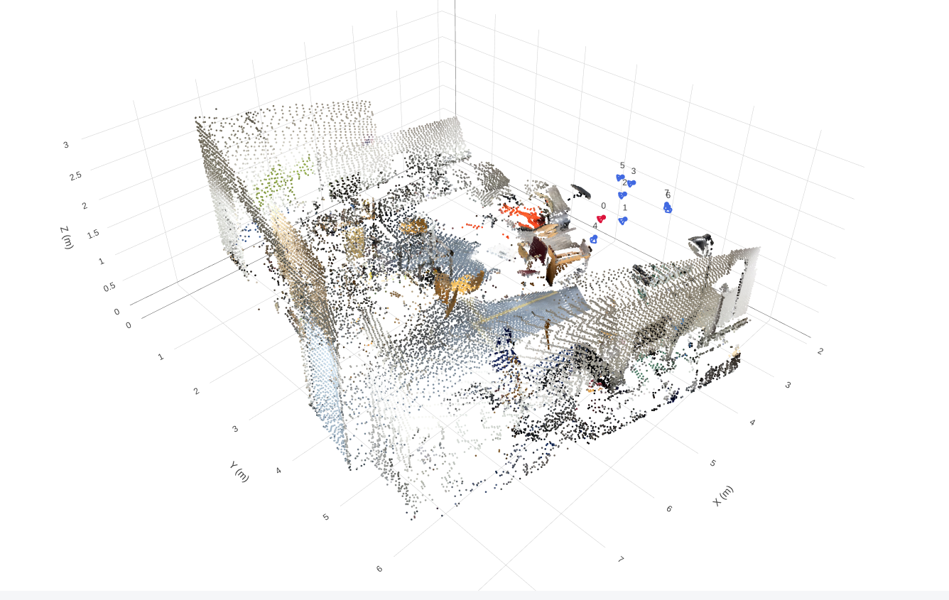
Unprojection screenshotdata/part1_unprojection.png
1.3. Canonicalization
I express every camera in the first sampled camera’s frame, then compute the distance of the valid-point centroid from the origin using the provided compute_scene_scale.
T0←i = (Tw←0)−1Tw←i
s = ‖mean(Xreference, valid)‖2
t′ = trelative/s,
z′ = z/s,
X′ = Xreference/s.
I divide translations, depth and points by the same scale without subtracting the centroid. Camera 0 therefore remains identity, and the valid-point centroid has distance approximately 1 from the origin. Rotations and intrinsics are unchanged.
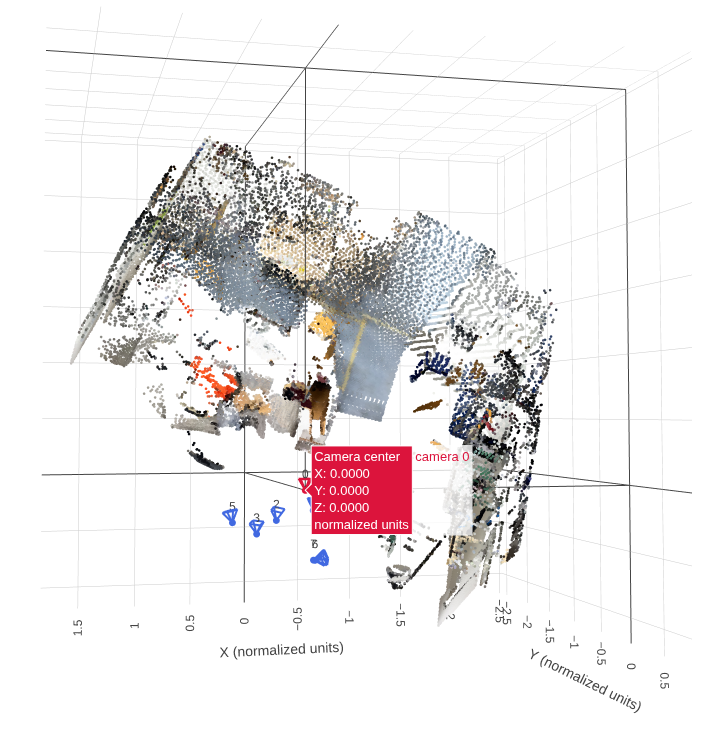
Canonicalization screenshotdata/part1_canonicalization.png
Show camera 0’s center and the valid-point centroid distance.
1.4. Camera Rays
Each ray starts at the camera center. I rotate the back-projected pixel direction into the canonical world frame and normalize it:
o = t′, d = RK−1[u, v, 1]T / ‖RK−1[u, v, 1]T‖2.
Translation determines the origin but is not added to the direction. All pixels in a view share the same origin; their unit directions vary with pixel position.
1.5. Plücker Coordinates
m = o × d, ℓ = [dx, dy, dz, mx, my, mz].
The direction describes the line’s orientation, while the moment encodes its offset from the coordinate origin. Moving o along the same line leaves m unchanged. For unit d, ‖m‖ is the line’s distance to the origin, and d · m = 0.
1.6. Dataloader
Training samples random views and calls my geometry functions; the first sampled view is camera 0. Validation and test use fixed prepared views with frame 0 as reference, recompute scale after sampling, and bypass my Q1 implementation.
Geometry functions return channel-last maps. The loader converts them to channel-first tensors and adds the batch dimension. Depth validity does not mask RGB.
1.7. Check Results
Checks on four training samples should report point/ray reprojection errors below 0.01 pixels and a valid-point centroid distance approximately equal to 1.
{
          "split": "train",
          "dataset_samples": 224,
          "checked_samples": 4,
          "samples": [
            {
              "sequence_name": "e050c15a8d_frame_007080",
              "views": 8,
              "resolution": 224,
              "valid_depth_fraction": 0.9779127240180969,
              "max_reprojection_error_px": 0.00010844774078577757,
              "max_ray_reprojection_error_px": 9.281559323426336e-05,
              "centroid_distance": 1.0
            },
            {
              "sequence_name": "5f99900f09_frame_002820",
              "views": 8,
              "resolution": 224,
              "valid_depth_fraction": 0.9903116226196289,
              "max_reprojection_error_px": 0.00012302029062993824,
              "max_ray_reprojection_error_px": 0.0001373291015625,
              "centroid_distance": 0.9999999403953552
            },
            {
              "sequence_name": "47b37eb6f9_frame_002720",
              "views": 8,
              "resolution": 224,
              "valid_depth_fraction": 0.9609947800636292,
              "max_reprojection_error_px": 9.073573164641857e-05,
              "max_ray_reprojection_error_px": 8.897326188161969e-05,
              "centroid_distance": 1.0
            },
            {
              "sequence_name": "4c5c60fa76_frame_006690",
              "views": 8,
              "resolution": 224,
              "valid_depth_fraction": 0.7516716122627258,
              "max_reprojection_error_px": 0.00010111196752404794,
              "max_ray_reprojection_error_px": 9.5367431640625e-05,
              "centroid_distance": 0.9999999403953552
            }
          ],
          "batch_shapes": {
            "rgb": [
              2,
              8,
              3,
              224,
              224
            ],
            "depth": [
              2,
              8,
              1,
              224,
              224
            ],
            "depth_valid": [
              2,
              8,
              1,
              224,
              224
            ],
            "K": [
              2,
              8,
              3,
              3
            ],
            "frame_numbers": [
              2,
              8
            ],
            "T_world_from_camera": [
              2,
              8,
              4,
              4
            ],
            "original_world_from_reference": [
              2,
              4,
              4
            ],
            "scene_scale": [
              2
            ],
            "points_world": [
              2,
              8,
              3,
              224,
              224
            ],
            "ray_origins": [
              2,
              8,
              3,
              224,
              224
            ],
            "ray_directions": [
              2,
              8,
              3,
              224,
              224
            ],
            "plucker": [
              2,
              8,
              6,
              224,
              224
            ]
          }
        }
I checked four training samples, each containing eight views at 224 × 224 resolution. The maximum point and ray reprojection errors were 0.000123 px and 0.000137 px, respectively, both well below 0.01 px. All valid-point centroid distances were approximately 1, and the batch shapes matched the expected dimensions.
Canonicalization. I transform the cameras and 3D points into the first camera's coordinate frame, then divide camera translations, depths and points by a shared scene scale. The first camera therefore has an identity pose, and the valid-point centroid lies approximately one unit from the origin. This provides consistent coordinate and scale conventions across samples.
World-space ray directions.
I compute each pixel's camera-space direction using the inverse intrinsics,
rotate it into the canonical world frame, and normalize it:
d = R K−1[u, v, 1]T /
        ‖R K−1[u, v, 1]T‖
.
The ray origin is the camera center, o = t.
Rotation determines the ray's orientation, while translation determines its origin.
Plücker moment.
I represent each ray using six channels, (d, m),
with direction followed by moment, where m = o × d.
The moment encodes the line's position relative to the coordinate origin
and remains unchanged if I choose another point along the same ray.
2. Novel-View Synthesis with Mini-LVSM
2.0. Implementation
I use source RGB images and source/target Plücker rays to predict target RGB images. Target RGB is used only for supervision.
Patches and tokens. I split each image into non-overlapping p × p patches in row-major order, flattening each patch in (row, column, channel) order. Unpatchify reverses this operation. I project source RGB (scaled to [−1, 1]) concatenated with its six ray channels, and project target rays separately.
I add shared 2D sinusoidal positional embeddings and concatenate all source tokens with one target's query tokens. Each target forms its own sequence:
N = (H / p)(W / p), tokens: (B · T, (S + 1) · N, D).
Prediction and loss. I apply input normalization and full-attention transformer blocks, retain the target-query tokens, then apply output normalization, the RGB head, sigmoid and unpatchify. The output shape is (B, T, 3, H, W). I average MSE over all target views, channels and pixels. When AMP is enabled, I use bfloat16 autocast for the forward pass and compute the loss in float32.
LMSE = (1 / M) ∑j=1M (ŷj − yj)2, M = B · T · 3 · H · W.
2.1. Overfitting
I use one fixed batch for 2,000 optimization steps to check whether the model can memorize the target images.
Final overfit PSNR: 36.54 dB.
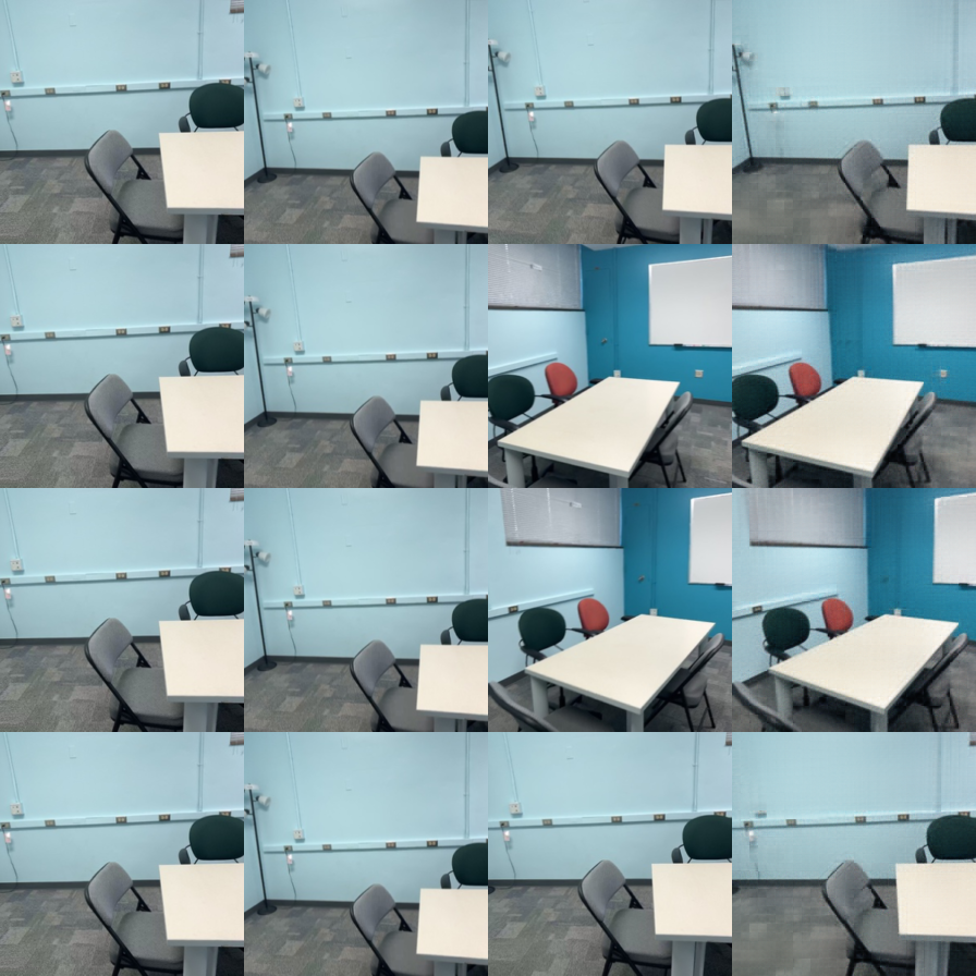
Image pending: data/part2_overfit.png
Observation: [Add the final loss, whether PSNR reaches approximately 30 dB, and any remaining visual errors.]
2.2. Training and Evaluation
Training settings. The values below are the provided configuration defaults, not a record of my completed run. I will confirm them against my saved configuration and replace any changed values.
| Setting | Value to confirm |
|---|---|
| Training / validation scenes | 224 / 28 |
| Input resolution / total sampled views | 224 × 224 / 8 |
| Training source / target views | 2 / 6 |
| Patch size / width / transformer layers | 8 / 384 / 8 |
| Batch size / configured epochs | 4 / 100 |
| Completed epochs | 100 |
| Initial learning rate / weight decay | 0.0002 / 0.05 |
| Optimizer β / warmup / gradient clipping | (0.9, 0.95) / 200 steps / 1.0 |
| AMP / seed | bfloat16 / 825 |
| Evaluation split / prepared-frame prefix | Validation / first 32 frames |
| Baseline loss / checkpoint | MSE / outputs/lvsm/best.pt |
Provided Mini-LVSM configuration
Training curves and visualization

Image pending: data/part2_training_curves.png
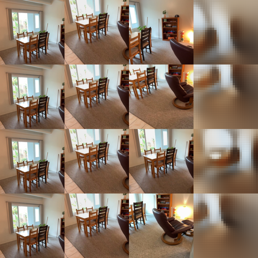
Image pending: data/part2_training_prediction.png
Validation ablations
I evaluate the same baseline checkpoint with 1, 2 and 4 source views. Correct conditioning uses the true target rays; shuffled conditioning uses another target view's rays; none uses zero target rays. PSNR (dB) and SSIM are higher-is-better metrics.
| Source views | Target rays | PSNR ↑ (dB) | SSIM ↑ |
|---|---|---|---|
| 1 | correct | 15.0690 | 0.5593 |
| 1 | shuffled | 11.7347 | 0.4905 |
| 1 | none | 12.3546 | 0.5406 |
| 2 | correct | 15.9193 | 0.5586 |
| 2 | shuffled | 11.4769 | 0.4762 |
| 2 | none | 12.3090 | 0.5373 |
| 4 | correct | 16.5731 | 0.5724 |
| 4 | shuffled | 11.6765 | 0.4808 |
| 4 | none | 12.3481 | 0.5478 |
Discussion
Source-view count. With correct target rays, I obtain PSNR values of 15.0690, 15.9193 and 16.5731 dB with 1, 2 and 4 source views, respectively. PSNR increases by 0.8504 dB from 1 to 2 sources and by another 0.6537 dB from 2 to 4 sources. This is consistent with additional views providing useful scene information. SSIM is not strictly monotonic: it changes from 0.5593 to 0.5586, then increases to 0.5724. Thus, more sources improve pixel fidelity in these settings, but do not improve every metric at every step.
Target-ray conditioning. I observe substantially better performance with correct rays at every source count. With 2 sources, shuffling the target rays reduces PSNR from 15.9193 to 11.4769 dB and SSIM from 0.5586 to 0.4762. Zeroing the rays gives 12.3090 dB and 0.5373 SSIM. Incorrect rays are more harmful than absent rays in all three source-count settings, suggesting that misleading viewpoint information disrupts prediction more than removing it. Without correct rays, PSNR stays near 11.5–11.7 dB for shuffled rays and 12.3–12.4 dB for zero rays as sources increase. Additional source images therefore do not compensate for incorrect target-view conditioning.
Limitations. I evaluate the same checkpoint throughout, so these experiments measure inference-time behavior rather than the effect of retraining with different source counts. The number of evaluated target images changes from 196 to 168 to 112 for 1, 2 and 4 sources, respectively, so the source-count comparison does not use identical target sets. Within each source count, the ray ablations use the same number of target images. The reported metrics establish quantitative differences; I do not infer visual sharpness from them alone.
2.3. Bonus: MSE + 0.1 L1
Question. Does adding L1 supervision to MSE improve validation PSNR, SSIM or visual sharpness?
I add a mean absolute error term over the same target RGB values:
LL1 = (1 / M) ∑j=1M |ŷj − yj|,
Lbonus = LMSE + 0.1 LL1.
Experimental settings. I compare the MSE baseline with MSE + 0.1 L1 over 100 epochs. Each validation pass evaluates 168 target images. I compare validation PSNR and SSIM, whose definitions are unchanged by the training loss, and select each run’s epoch with the highest validation PSNR. The logs do not record the full configurations, so they alone cannot verify identical initialization, optimizer or data-sampling settings.

Image pending: data/part2_bonus_curves.png
| Training loss | Selected epoch (0-based) | Validation PSNR ↑ (dB) | Validation SSIM ↑ |
|---|---|---|---|
| MSE | 98 | 15.9193 | 0.5586 |
| MSE + 0.1 L1 | 97 | 16.0709 | 0.5608 |
Results. I obtain 16.0709 dB PSNR and 0.5608 SSIM with MSE + 0.1 L1 at epoch 97, compared with 15.9193 dB and 0.5586 for MSE at epoch 98. This is a gain of 0.1516 dB PSNR and 0.0022 SSIM. At the final epoch, the combined loss also performs better: 16.0578 versus 15.9121 dB, and 0.5600 versus 0.5569 SSIM. The curves indicate a small late-training benefit rather than a large improvement.
Explanation. MSE penalizes large residuals quadratically, while L1 supplies a constant-magnitude gradient for nonzero residuals. Adding L1 changes the relative emphasis on small and large pixel errors. It may affect image detail, but improvement in sharpness, PSNR or SSIM must be established by the measured results.
Conclusion and limitations. Adding 0.1 L1 produces a modest improvement in both validation metrics in these runs. The final-epoch comparison supports the same trend as checkpoint selection. However, one run per loss and one L1 weight are insufficient to establish statistical reliability or identify the best weight. I cannot conclude that images are sharper without inspecting matched predictions. I do not compare total loss values directly because the two objectives have different definitions.
3. Multi-View Geometry with Mini-VGGT
3.0. Implementation
I use frozen DINO features and alternate within-view and cross-view attention to predict cameras, depth and confidence. I supervise the camera and depth heads using canonicalized targets. For visualization, I reconstruct point clouds from the predicted cameras and depth rather than predicting point maps directly.
3.1. Overfitting
I fit one fixed training clip to check the implementation before full training.

Image pending: data/part3_overfit_loss.png
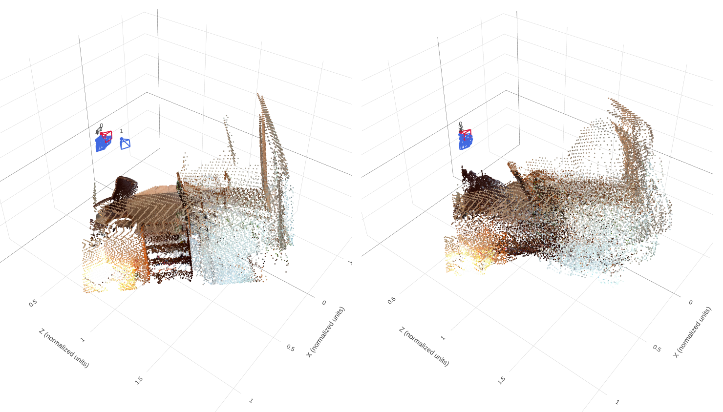
Image pending: data/part3_overfit_geometry.png
Observation. I observe that the predicted point cloud captures the main layout and color distribution of the fixed scene. However, it remains thicker and less clearly structured than the ground truth, with blurred boundaries and imperfect alignment between surfaces. The predicted camera centers also appear more tightly clustered than the GT cameras. These differences suggest that the model has learned the overall scene structure but has not fully reproduced its depth and relative camera positions.
3.2. Training and Evaluation
Training settings
Training settings
I train Mini-VGGT with 8 input views sampled from a 32-frame window, using 224 × 224 images and a batch size of 4.
| Setting | Value |
|---|---|
| Encoder | Frozen DINOv2 ViT-B/14 |
| Input views / sampling range | 8 / 32 frames |
| Image resolution | 224 × 224 |
| Frame/global attention pairs | 8 pairs (16 blocks) |
| Embedding dimension / attention heads | 384 / 6 |
| Direct point-map prediction | Disabled |
| Batch size / data workers | 4 / 8 |
| Configured training epochs | 300 |
| Initial learning rate | 0.0006 |
| Weight decay | 0.01 |
| Warmup epochs | 10 |
| Minimum learning-rate ratio | 0.05 |
| Camera / depth loss weights | 5.0 / 1.0 |
| Evaluation frame prefix | First 32 prepared frames |
| Checkpoint selection | Lowest validation loss |
Ltotal = 5 Lcamera + Ldepth.
Normal-training loss curve

Image pending: data/part3_training_loss.png
Validation and test metrics
I evaluate the same checkpoint, outputs/vggt_train/best.pt,
on the full validation and test splits without a batch limit.
Each split contains 28 scenes and 784 camera pairs, with no degenerate
GT translation pairs.
| Metric | Validation | Test |
|---|---|---|
| Depth AbsRel ↓ | 0.1638 | 0.1873 |
| Depth δ1 ↑ | 0.7751 | 0.7314 |
| Rotation AUC@5° ↑ | 0.1314 | 0.1722 |
| Rotation AUC@15° ↑ | 0.4210 | 0.4512 |
| Rotation AUC@30° ↑ | 0.6180 | 0.6679 |
| Translation AUC@5° ↑ | 0.0066 | 0.0026 |
| Translation AUC@15° ↑ | 0.0469 | 0.0288 |
| Translation AUC@30° ↑ | 0.1308 | 0.1167 |
| Joint pose AUC@5° ↑ | 0.0023 | 0.0010 |
| Joint pose AUC@15° ↑ | 0.0304 | 0.0196 |
| Joint pose AUC@30° ↑ | 0.1105 | 0.1028 |
Depth metrics use all GT-valid pixels. All AUC values range from 0 to 1. Translation AUC allows sign ambiguity, and joint pose AUC uses the larger rotation or translation-direction error for each camera pair.
Discussion
Depth generalization. I obtain a depth AbsRel of 0.1638 on validation and 0.1873 on test. Depth δ1 decreases from 77.51% to 73.14%, indicating weaker depth accuracy on the test scenes. Differences in scene content, visibility and surface appearance may contribute to this gap, although the aggregate metrics alone do not identify its cause.
Camera estimation. I observe better rotation accuracy on test: Rotation AUC@30° increases from 0.6180 to 0.6679, while mean rotation error decreases from 15.71° to 11.11°. Translation direction remains difficult on both splits, with mean errors of 47.44° and 47.28°. Despite similar mean translation errors, test Translation AUC@30° is lower (0.1167 versus 0.1308), indicating poorer performance within the evaluated angular thresholds.
Overall limitations. Translation estimation remains a major bottleneck, with joint pose AUC@30° of only 0.1105 on validation and 0.1028 on test. Relative camera errors can misalign reconstructed depth maps, producing inconsistent multi-view geometry even when individual depth maps capture the scene reasonably well. The mixed changes across depth and rotation metrics show that neither split is uniformly easier across all tasks.
Geometry on four held-out scenes
I compare GT and predicted geometry for four different held-out scenes, using matched viewing angles and showing both point clouds and camera poses.
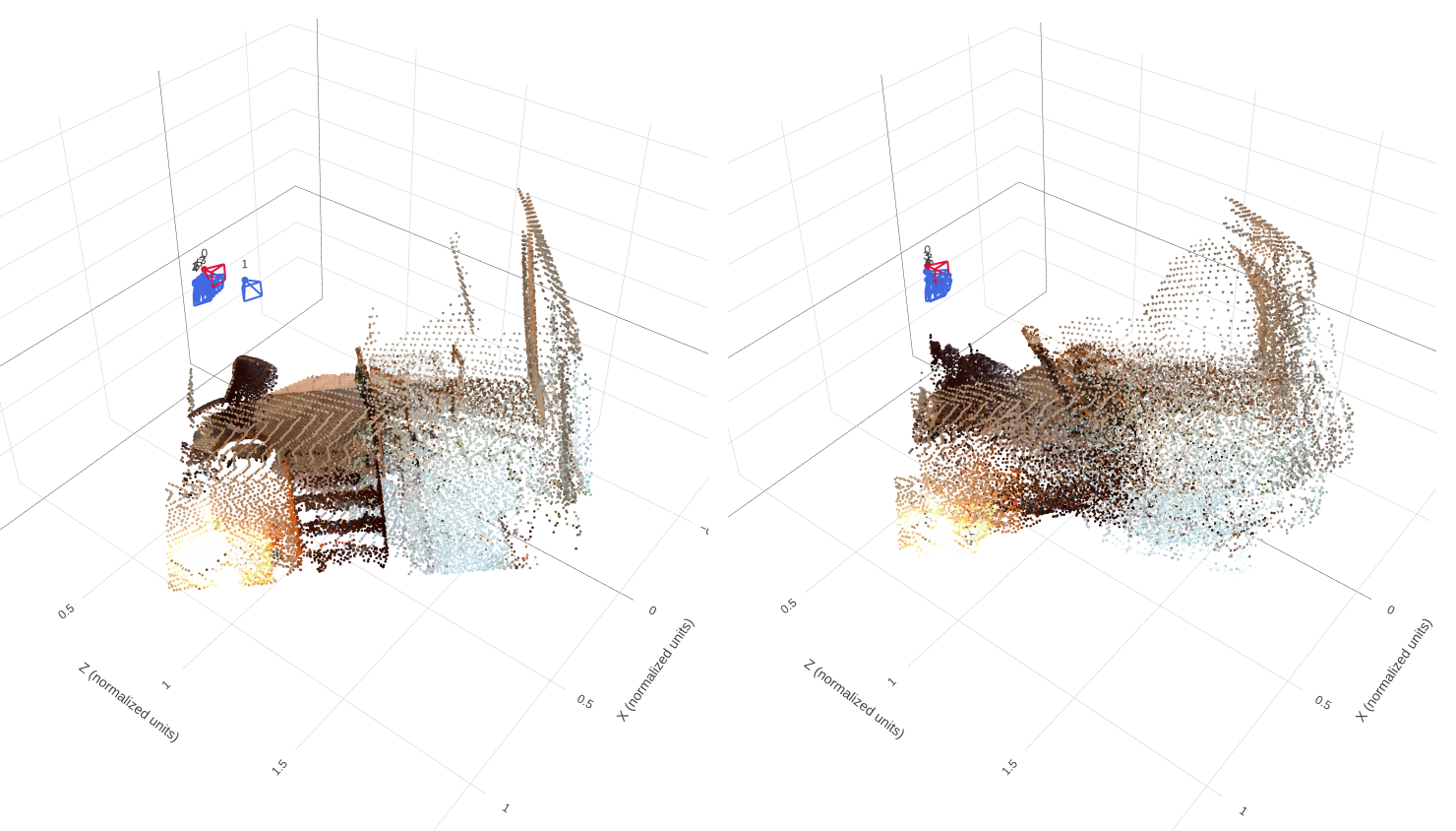
Image pending: data/part3_scene1_geometry.png
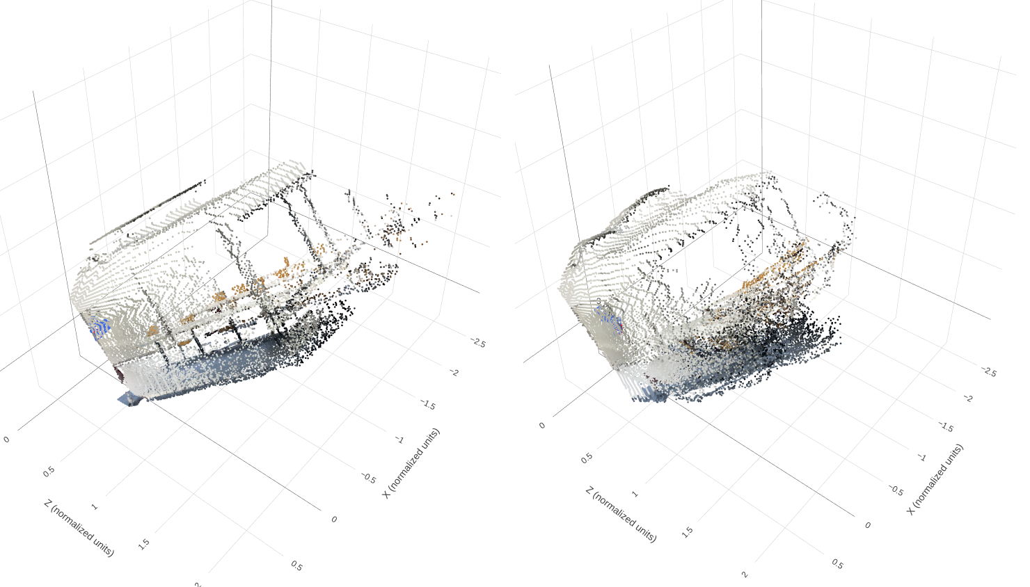
Image pending: data/part3_scene2_geometry.png
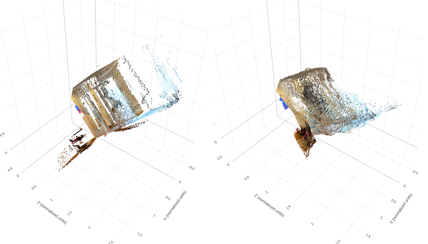
Image pending: data/part3_scene3_geometry.png
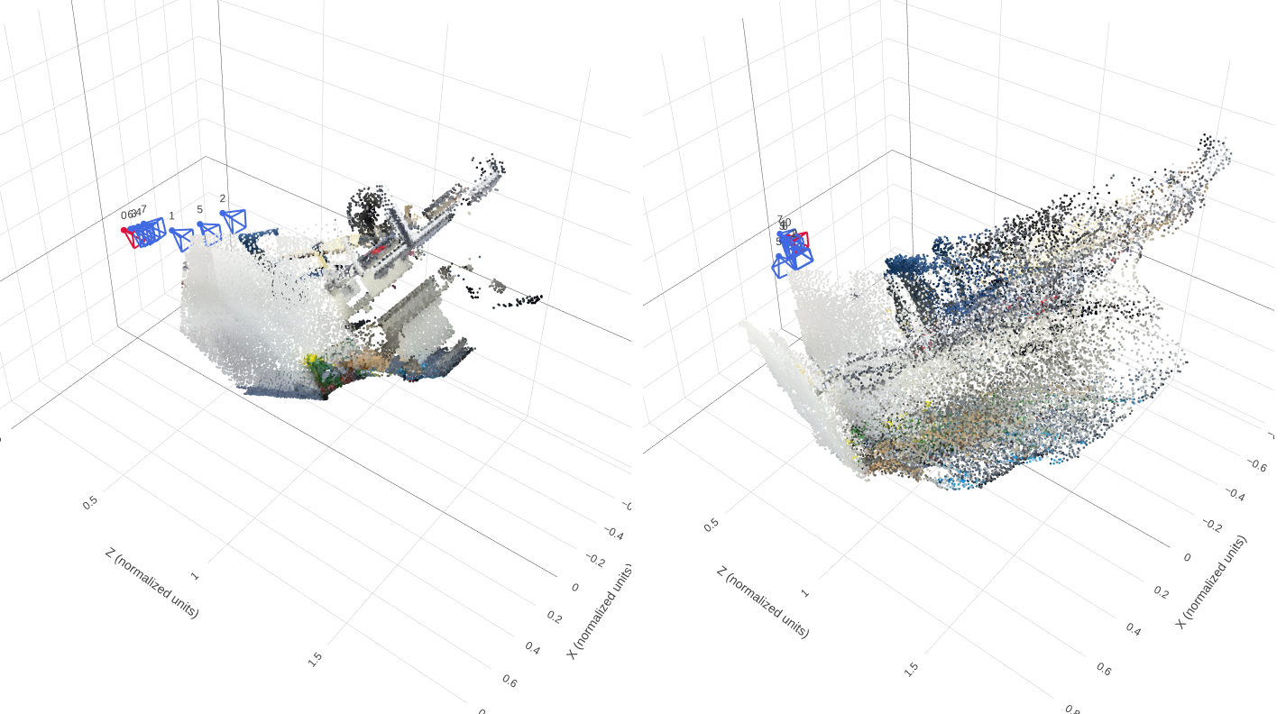
Image pending: data/part3_scene4_geometry.png
Discussion
Depth and surfaces. I observe that the predictions recover the broad scene layout and color distribution, but some surfaces appear thicker, distorted or less clearly separated than in GT. In the room example with the brown furniture and light-colored wall, the prediction loses clear surface boundaries. In the elongated room example, the reconstructed geometry is more compressed and does not preserve the full spatial extent of GT. In the example with the rectangular frame and blue region, narrow structures become less distinct and neighboring surfaces blend together. These observations indicate imperfect depth and multi-view alignment; the screenshots alone cannot separate their contributions.
Camera estimation. I obtain Rotation AUC@30° values of 0.6180 on validation and 0.6679 on test, whereas Translation AUC@30° is only 0.1308 and 0.1167. Joint pose AUC@30° remains low at 0.1105 and 0.1028, respectively. Translation direction is therefore a major limitation. In the brown-furniture example, the predicted camera centers appear more tightly clustered than the GT cameras, consistent with an inaccurate relative camera configuration. Camera errors may contribute to the thickened and misaligned surfaces, although depth errors can produce similar artifacts.
Held-out generalization. I obtain worse depth accuracy on test than on validation: AbsRel increases from 0.1638 to 0.1873, while δ1 decreases from 77.51% to 73.14%. Rotation accuracy improves on test, but translation and joint pose AUC decrease at all reported thresholds. Neither split is therefore uniformly easier across tasks. The qualitative examples show that preserving surface boundaries and the spatial extent of the scene remains challenging. Limited training data, ambiguous visual correspondences and differences in scene appearance are possible explanations, but these experiments do not isolate their effects.
3.3. Bonus: Number of Input Views
Question. How does evaluating with 2, 4 or 8 input views affect depth/pose accuracy, runtime and GPU memory?
Experimental settings. I compare the same checkpoint on the full validation split at 224 × 224 resolution, with seed 825, the first 32 prepared frames and evaluation batch size 1. Only the input view count changes.
| Views | AbsRel ↓ | δ1 ↑ | Rotation AUC@30° ↑ | Translation AUC@30° ↑ | Joint pose AUC@30° ↑ |
|---|---|---|---|---|---|
| 2 | 0.1234 | 0.8528 | 0.6429 | 0.1488 | 0.1143 |
| 4 | 0.1549 | 0.7742 | 0.6095 | 0.1597 | 0.1288 |
| 8 | 0.1638 | 0.7751 | 0.6183 | 0.1308 | 0.1105 |

Results. I do not observe a monotonic improvement with more input views. With 2 views, I obtain the lowest AbsRel (0.1234), highest δ1 (0.8528) and highest Rotation AUC@30° (0.6429). With 4 views, I obtain the best Translation AUC@30° (0.1597) and joint pose AUC@30° (0.1288). Increasing to 8 views does not improve these metrics, although normalized depth RMSE is lowest with 8 views (0.2082). In the qualitative comparison, additional views produce a denser combined point cloud, but the surfaces remain thick and imperfectly aligned. Greater point density alone does not establish better reconstruction accuracy. Runtime and GPU memory were not recorded, so I cannot quantify their changes.
Possible explanations. Additional views provide more scene observations, but errors in predicted depth and relative camera poses can prevent those observations from aligning consistently. More views also introduce additional camera pairs, potentially including more difficult viewpoint relationships. These factors may explain why additional inputs do not consistently improve the aggregate metrics. The denser point clouds partly reflect the larger number of predicted depth maps being combined.
Conclusion and limitations. I find that 2 views perform best for relative depth accuracy and rotation AUC@30°, while 4 views perform best for translation and joint pose AUC@30°. No setting is best across all metrics, and I cannot determine the best accuracy/cost tradeoff without timing and memory measurements. This is an inference-time comparison using the same checkpoint trained with 8 views. Changing the view count changes the evaluated pixels (2,588,890 / 5,168,551 / 10,347,720) and camera pairs (28 / 168 / 784), and may also change sampled frames and scene normalization. The results therefore compare complete evaluation settings rather than isolating the effect of adding context to identical target views.