Carnegie Mellon University · 16-825 Learning for 3D Vision

Single View to 3D

Assignment 2 report for voxel, point-cloud, mesh, implicit, and parametric 3D reconstruction from a single RGB image.

Name: Guo Yu Assignment 2

Submission checklist

✓ Q1.1 voxel fitting visualization
✓ Q1.2 point-cloud fitting visualization
✓ Q1.3 mesh fitting visualization
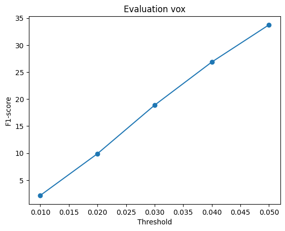
✓ Q2.1 three voxel examples + F1@0.05 + F1 curve
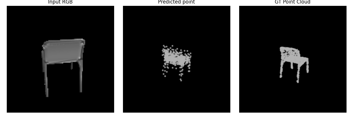
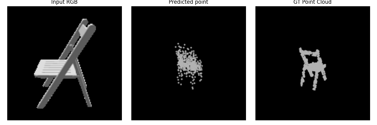
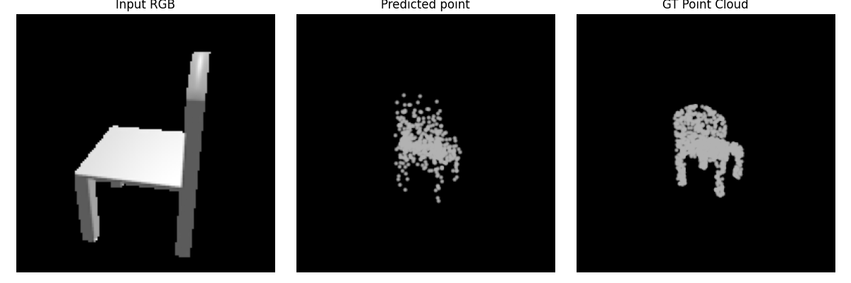
✓ Q2.2 three point examples + F1@0.05 + F1 curve
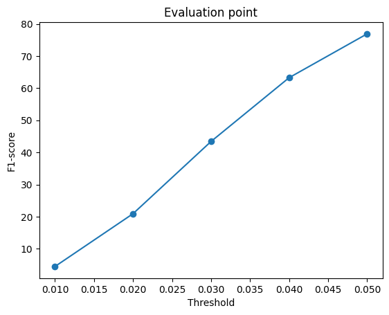
✓ Q2.3 three mesh examples + F1@0.05 + F1 curve
✓ Quantitative voxel / point / mesh comparison
✓ Q2.4 hyperparameter experiment + conclusion
✓ Q2.5 interpretation visualization
✓ At least one Q3 extension

1. Exploring Loss Functions

10 points

1.1 Fitting a Voxel Grid

4 pts

Requirement. Implement binary cross-entropy voxel loss, optimize a source voxel grid toward the target, and visualize optimized vs. ground-truth voxel grids.

python fit_data.py --type 'vox'
Voxel fitting result
Optimized voxel grid vs. ground truth
BCE Loss.
loss = F.binary_cross_entropy_with_logits(voxel_src, voxel_tgt.squeeze(1).float())

1.2 Fitting a Point Cloud

3 pts

Requirement. Implement Chamfer distance yourself (KNN utilities are allowed), fit a source point cloud to a target, and visualize the result.

python fit_data.py --type 'point'
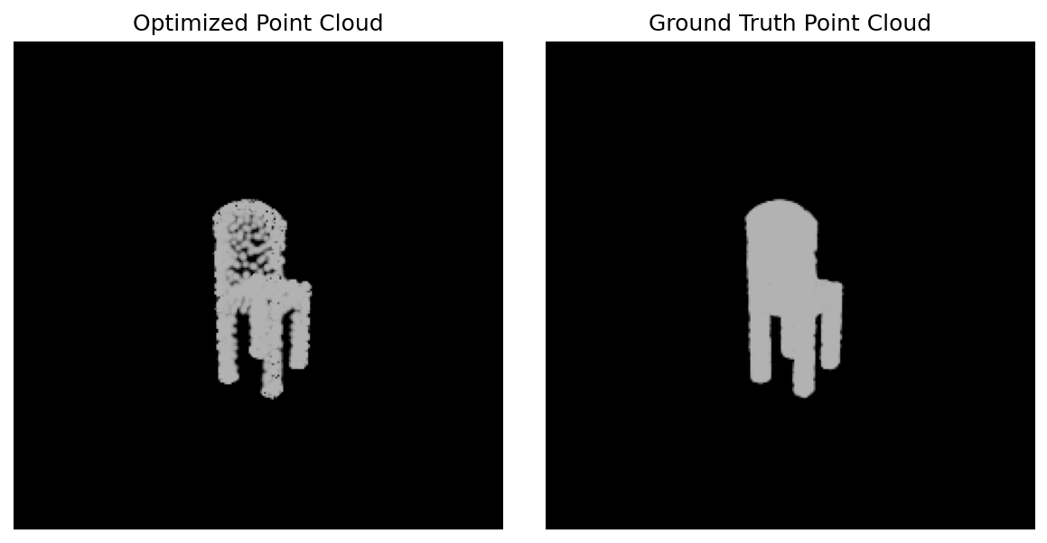
Point fitting result
Optimized point cloud vs. ground truth
Chamfer loss.
dists_src_to_tgt, _, _ = knn_points(point_cloud_src, point_cloud_tgt, K=1)
dists_tgt_to_src, _, _ = knn_points(point_cloud_tgt, point_cloud_src, K=1)
loss_src = torch.mean(dists_src_to_tgt)
loss_tgt = torch.mean(dists_tgt_to_src)
loss_chamfer = loss_src + loss_tgt

1.3 Fitting a Mesh

3 pts

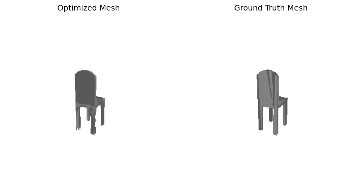
Requirement. Add a mesh smoothness loss, optimize the source mesh, and show optimized vs. ground-truth meshes.

python fit_data.py --type 'mesh'
Mesh fitting result
Optimized mesh vs. ground truth
Smoothness loss.
loss_laplacian = mesh_laplacian_smoothing(mesh_src, method="uniform")

2. Reconstructing 3D from a Single View

80 points
The report layout below follows the required webpage deliverables: three test examples for each representation, F1@0.05, F1 plots, a cross-representation comparison, a hyperparameter experiment, and an interpretation section.
Precomputed ResNet18 image features were used with --load_feat during training and evaluation.

2.1 Image → Voxel Grid

20 pts
python train_model.py --type 'vox'
python eval_model.py --type 'vox' --load_checkpoint
Voxel size
32³
Loss
BCE

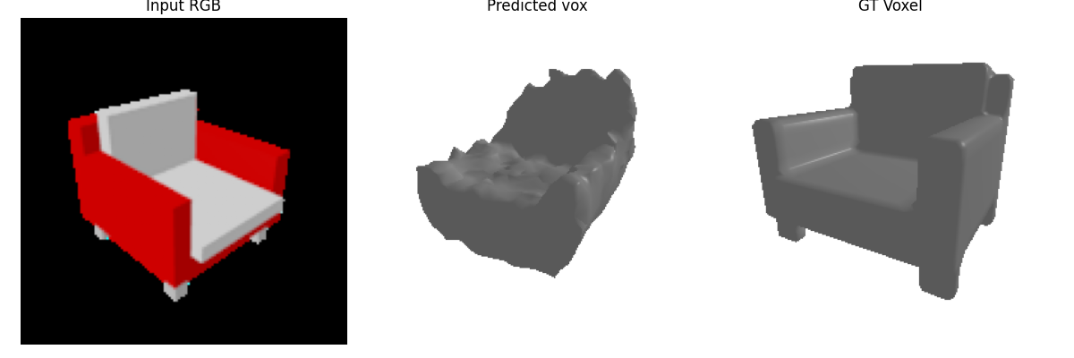
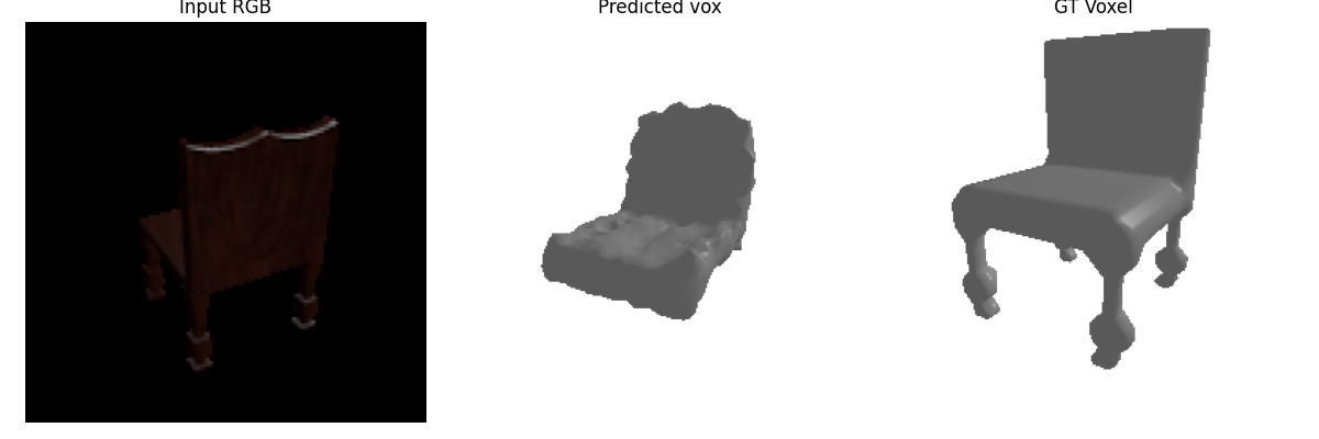
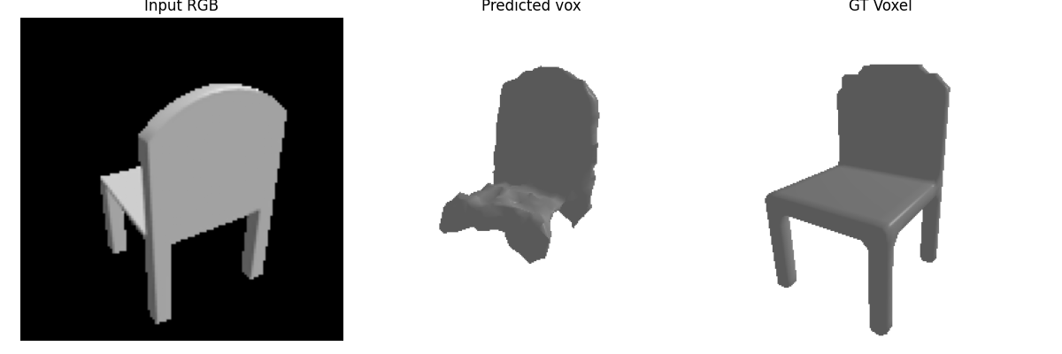
Three test examples

Voxel example 1
Example 1 · Input / Prediction / GT
Voxel example 2
Example 2 · Input / Prediction / GT
Voxel example 3
Example 3 · Input / Prediction / GT

F1 curve

Voxel F1 plot
F1 score across distance thresholds

2.2 Image → Point Cloud

20 pts
python train_model.py --type 'point'
python eval_model.py --type 'point' --load_checkpoint
# Points
1024
Loss
Chamfer

Three test examples

Point example 1
Example 1 · Input / Prediction / GT
Point example 2
Example 2 · Input / Prediction / GT
Point example 3
Example 3 · Input / Prediction / GT

F1 curve

Point F1 plot
F1 score across distance thresholds

2.3 Image → Mesh

20 pts
python train_model.py --type 'mesh'
python eval_model.py --type 'mesh' --load_checkpoint
Init mesh
Ico sphere

Three test examples

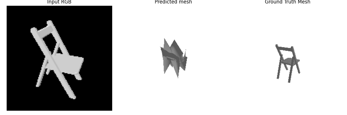
Mesh example 1
Example 1 · Input / Prediction / GT
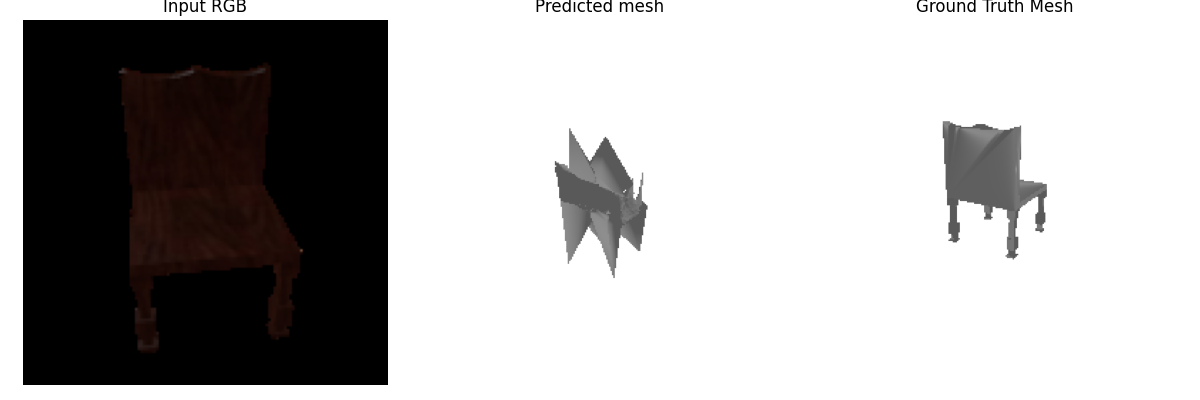
Mesh example 2
Example 2 · Input / Prediction / GT
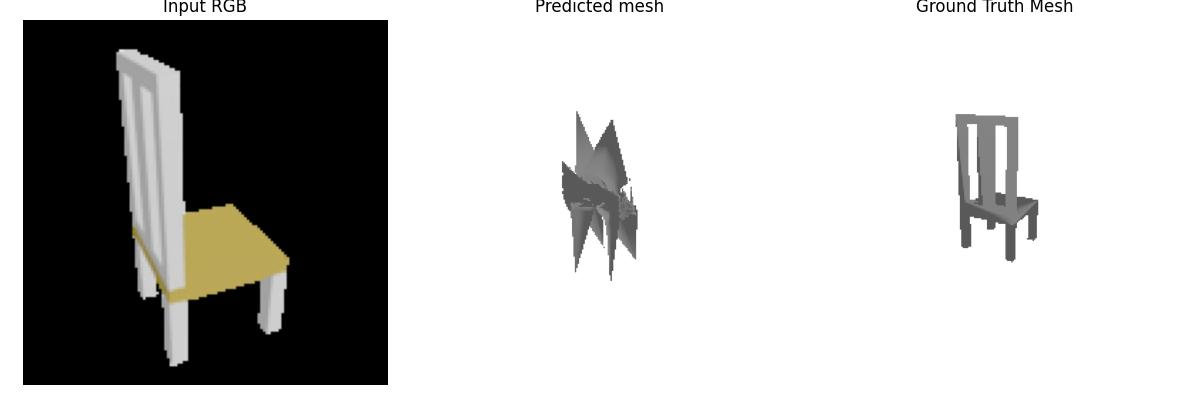
Mesh example 3
Example 3 · Input / Prediction / GT

F1 curve

Mesh F1 plot
F1 score across distance thresholds

2.4 Hyperparameter Analysis

10 pts

Requirement. Vary one meaningful hyperparameter and provide a conclusive analysis. Examples from the assignment include n_points, voxel size, Chamfer weight, or initial mesh.

Conclusion I experimented with several hyperparameters, including the number of sampled points n_points, the Chamfer loss weight w_chamfer, and the learning rate. Increasing n_points did not lead to a clear improvement in reconstruction quality. Although denser point sampling slightly increased the numerical coverage of the predicted surface, the qualitative geometry remained similar, and the additional points mainly made the point cloud denser rather than more structurally accurate. Changing w_chamfer also had limited effect. Since Chamfer distance was already the dominant reconstruction objective, moderate changes to its weight did not substantially alter the learned shape. The model tended to converge to similar solutions unless the relative weighting was changed aggressively. In contrast, reducing the learning rate produced a more noticeable improvement. With a smaller learning rate, the optimization became more stable and the reconstructed geometry was less noisy, especially in later training stages. This suggests that, for this model, optimization stability had a larger influence on the final reconstruction quality than simply increasing point density or rescaling the Chamfer loss. Among the tested hyperparameters, learning rate had the most meaningful effect. Increasing model output resolution through more sampled points did not necessarily improve geometric structure, while a smaller learning rate helped the model converge more smoothly to a better reconstruction

2.5 Interpret Your Model

10 pts

Requirement. Create a visualization that provides insight beyond final predictions and scalar metrics.

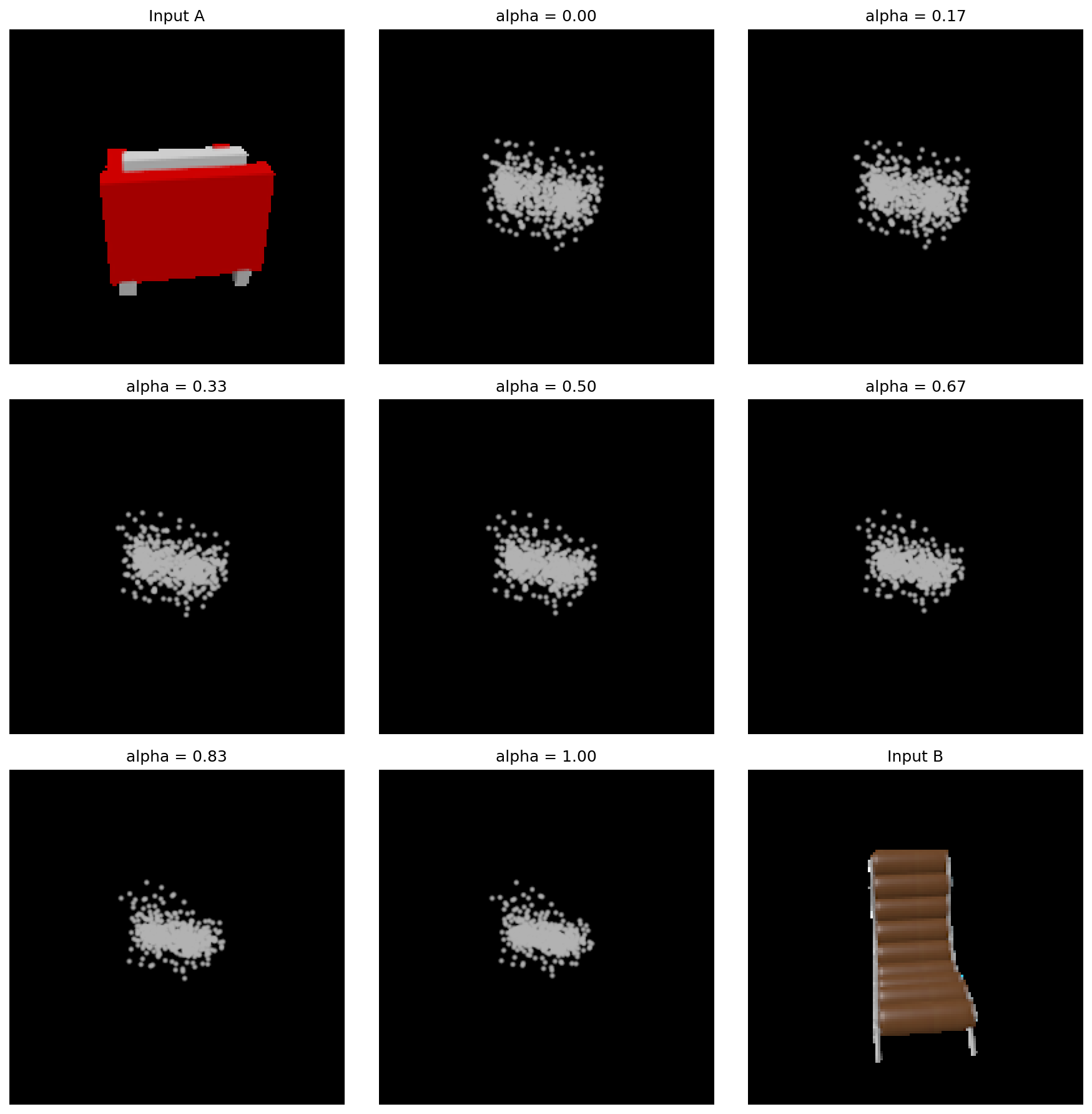
Model interpretation
Interpretation visualization
Linear Interpolation
To interpret the learned feature space, I linearly interpolated between the image features of two test examples and decoded the intermediate features into point clouds. As the interpolation coefficient changes from 0 to 1, the predicted point cloud changes gradually from the reconstruction associated with the first image toward that of the second image. This suggests that the learned representation is locally smooth, with intermediate feature vectors producing intermediate 3D geometries rather than abrupt changes in prediction. At the same time, some intermediate reconstructions appear blurred or averaged, indicating that a linear path in feature space does not always correspond to a realistic chair shape.

3. Exploring Other Architectures / Datasets

Choose ≥ 1 · 10 pts each

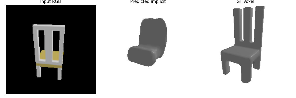
3.1 Implicit Network

10 pts

Requirement. Predict occupancy from an image feature and 3D coordinate, using a 32×32×32 meshgrid in normalized (-1,1)^3.

f(image_feature, x, y, z) → occupancy

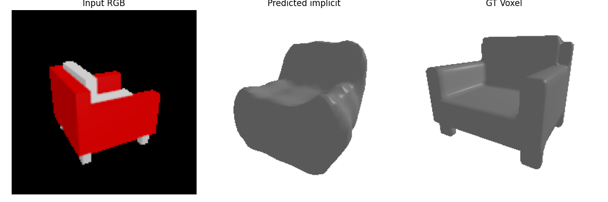
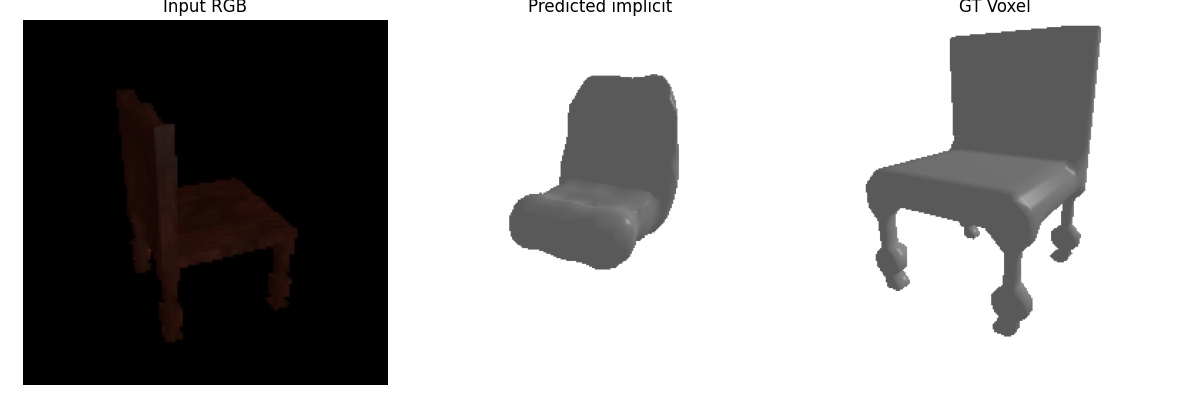
Three test examples

Implicit result 1
Implicit example 1 · Input / Prediction / GT
Implicit result 2
Implicit example 2 · Input / Prediction / GT
Implicit result 3
Implicit example 3 · Input / Prediction / GT

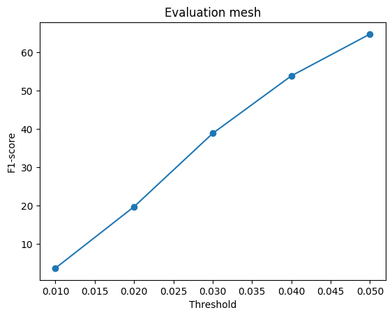
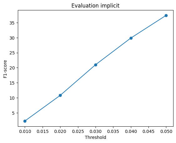
F1 curve

Implicit F1 plot
Implicit F1 score across distance thresholds
Analysis. The implicit model represents the 3D shape as an occupancy function conditioned on both the image feature and a queried 3D coordinate. For each input image, I construct a (32×32×32) grid of coordinates in the normalized space ([-1,1]^3). To provide the decoder with richer spatial information, each coordinate is augmented using sinusoidal positional encoding with frequencies 1, 2, 4, and 8, producing a 27-dimensional coordinate representation. This encoded coordinate is concatenated with the global image feature and passed through an MLP that predicts an occupancy logit for each spatial location. The final output is reshaped into a (32^3) occupancy grid. Compared with a conventional voxel decoder, this formulation makes occupancy explicitly dependent on spatial coordinates, allowing the network to learn a continuous coordinate-conditioned representation rather than directly decoding the entire voxel volume from a single feature vector.

3.2 Parametric Network

10 pts

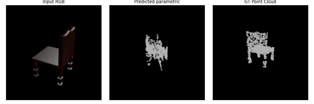
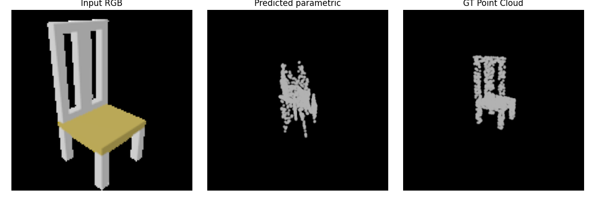
Requirement. Map sampled 2D parameter points to 3D points conditioned on the image.

f(image_feature, u, v) → (x, y, z)

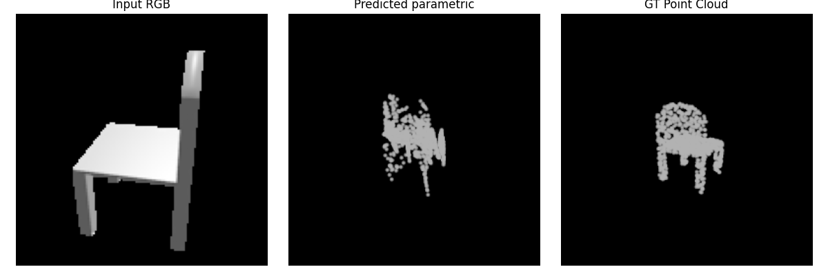
Three test examples

Parametric result 1
Parametric example 1 · Input / Prediction / GT
Parametric result 2
Parametric example 2 · Input / Prediction / GT
Parametric result 3
Parametric example 3 · Input / Prediction / GT

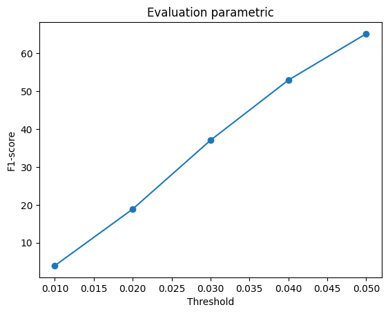
F1 curve

Parametric F1 plot
Parametric F1 score across distance thresholds
Analysis.The parametric model reconstructs the object by learning mappings from sampled 2D parameter coordinates to 3D points. I use eight independent parametric patches. For each patch, 2D points are randomly sampled from ([-1,1]^2), concatenated with the image feature, and passed through a separate MLP that predicts their corresponding 3D coordinates. The point sets generated by all eight patches are then concatenated to form the final reconstructed point cloud. Using multiple patches gives the model more flexibility than a single continuous 2D surface, since different patches can represent different parts of the object and do not need to maintain one global surface parameterization. This is especially useful for chair geometry, where the seat, back, and legs form several distinct structures that are difficult to represent accurately with only one parametric patch.

Implementation Notes

Pretrained features: Training and evaluation use the provided pretrained ResNet18 image features with --load_feat.