Assignment 3: Volume Rendering, NeRF, and 3D Gaussian Splatting
16-825 Learning for 3D Vision · Fall 2026 · Jinxi He (ginh)
I did all three NeRF extensions (4.1–4.3) and 7.1 for the Gaussian part. Unless a section says otherwise, Part A results are on the lego scene at 128×128 (4.1 uses the materials scene, as the handout asks), and PSNR means the average over the 200 test views at the final checkpoint.
A. Neural Volume Rendering
1.3 Ray Sampling (5 points)
get_pixels_from_image maps pixel centers to NDC with \( x = 2(i + 0.5)/W - 1 \) and then applies the starter's
sign flip, since PyTorch3D has +x pointing left and +y up. get_rays_from_pixels unprojects these points to
depth 1 with unproject_points, and the ray directions are the normalized vectors from the camera center to them.

grid.png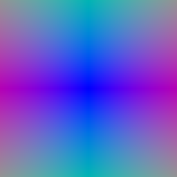
rays.png1.4 Point Sampling (5 points)
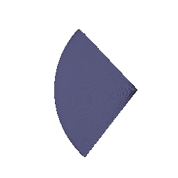
The sampler spaces n_pts_per_ray depths evenly between min_depth and max_depth and
returns origin + depth × direction for every ray.
1.5 Volume Rendering (20 points)
Each sample gets the weight \( w_i = T_i \left(1 - e^{-\sigma_i \delta_i}\right) \), where \( \delta_i \) is the distance to the next sample and \( T_i = \exp\big(-\sum_{j<i} \sigma_j \delta_j\big) \) is the transmittance up to it. Color and depth are the weighted sums \( \sum_i w_i c_i \) and \( \sum_i w_i z_i \). The depth map below is divided by its maximum.

part_1.gif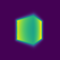
2.1–2.3 Optimizing a Basic Implicit Volume (5 + 5 points)
get_random_pixels_from_image picks n_pixels different pixels with torch.randperm, and
the loss is the MSE between rendered and ground-truth colors. After training:
box center (0.25, 0.25, 0.00), side lengths (2.00, 1.50, 1.50).
To get these I had to change one line of the starter. sample_images_at_xy calls grid_sample with
align_corners=True, but our rays go through pixel centers, which is the align_corners=False
convention. With True the ground-truth colors are read up to half a pixel off and the box comes out a bit too
large, (2.005, 1.504, 1.503), so the first side rounds to 2.01. With False the fit is exact to four decimals,
and a box with exactly these parameters reproduces the training images (146.5 dB).

part_2.gif (mine)
3 Optimizing a Neural Radiance Field (20 points)
The network is a smaller version of the one in the NeRF paper. The position is encoded with 6 harmonic frequencies and goes
through a 6-layer, 128-wide ReLU MLP, which gets the encoding again at layer 3. A linear layer with a ReLU gives the
density, and a small sigmoid head (128 → 64 → 3) gives the color. There is no view dependence yet. I kept the
training settings of nerf_lego.yaml: 128 samples per ray in [2, 6], 1,024 rays per batch, Adam at 5e-4 decayed
by 0.8 every 50 epochs, 250 epochs. Test PSNR: 24.55 dB.

part_3.gifOne problem I ran into: with PyTorch's default initialization the ReLU density is sometimes zero everywhere from the start (35 of 200 seeds, tested on 20,000 random points in the scene), and since no gradient gets through the ReLU, the network never trains. One of my 400×400 materials runs stayed black because of this. Xavier weights, zero biases and a bias of 0.1 on the density layer fixed it (none of 500 seeds starts dead in the same test). The model above uses this initialization; with the default one the same run got 24.23 dB.
4.1 View Dependence (+10 points)
For view dependence I encode the ray direction with 2 harmonic frequencies (15 values) and concatenate it with the 128-d
position feature right before the color head, as in the NeRF paper. The density still depends only on the position. All
runs below are on the materials scene for 250 epochs, at 128×128 (nerf_materials.yaml) and 400×400
(nerf_materials_highres.yaml).
| Materials | Train PSNR | Test PSNR | Train − test |
|---|---|---|---|
| No view dependence | 23.83 | 23.40 | 0.43 |
| Direction, 2 frequencies | 24.86 | 24.07 | 0.79 |
| Direction, 6 frequencies | 24.84 | 24.02 | 0.82 |
| Direction, 2 frequencies, 400×400 | 25.04 | 24.34 | 0.70 |


View dependence adds 0.67 dB on the test views. It is easiest to see on the shiny spheres: the highlights are brighter, while without view dependence they get averaged into the base color.
The price is more overfitting. The test PSNR still goes up, but the train PSNR goes up more, so the gap between them almost doubles (0.43 → 0.79 dB): a color that depends on the direction can fit how each training view looks instead of learning one consistent material. 6 direction frequencies gave the same result as 2 (24.02 vs 24.07 dB on the test views, gap 0.82 dB; one run each, so these small differences are within noise). The overfitting probably stays small because the direction only enters the last, small color layer with a low-frequency encoding, so the color can only change slowly with the viewing angle, and because the density, and with it the geometry, is shared by all views.
4.2 Coarse/Fine Sampling (+10 points)
I use two networks with the Part 3 architecture (nerf_lego_coarse_fine.yaml). The coarse network is evaluated
at 64 evenly spaced samples. Its weights (detached) define a piecewise-constant PDF along the ray, and sample_pdf
draws 128 more depths from it by inverse-CDF sampling. The fine network then renders all 192 samples in sorted order, and
both renders get an MSE loss. At test time I take evenly spaced quantiles instead of random ones, so the renders are
deterministic.
| Lego, 128×128 | Test PSNR | Train step | Render one frame |
|---|---|---|---|
| Uniform, 128 samples (Part 3) | 24.55 | 16.3 ms | 147 ms |
| Coarse network alone, 64 samples | 23.33 | – | – |
| Coarse 64 + fine 128 | 24.89 | 32.4 ms (2.0×) | 257 ms (1.7×) |
| Uniform, 256 samples (same cost) | 24.95 | 31.9 ms (2.0×) | 271 ms (1.8×) |


The fine pass is better than the coarse network alone on every one of the 200 test views, by 1.56 dB on average and up to 2.4 dB. Thin parts get sharper: the bars of the cab, the gears on the tracks, the joints of the arm. Compared with Part 3 (uniform 128) the gain is 0.34 dB. It costs about 2× per training step, 1.7× per rendered frame and twice the parameters. The timings come from a shared GPU, so take them as rough; in other runs I measured 1.6–2.0× for both.
The fair comparison, though, is uniform sampling with 256 points, which also runs an MLP 256 times per ray, and it is just as good (24.95 vs. 24.89 dB). On this scene the depth range [2, 6] is short and the images are only 128×128, so 256 uniform samples (0.016 apart) already resolve the surfaces. I would expect importance sampling to pay off when the depth range is long compared with the objects, or at high resolution, where uniform sampling needs many more points to be as dense near the surfaces.
4.3 VolSDF (+10 points)
NeuralSurface uses the Part 3 backbone (6 harmonic frequencies, 6 layers of 128). The signed distance \( d \)
comes from a linear layer with no activation, and the color from a 2-layer sigmoid head on the same features. The network
starts as the SDF of a unit sphere (the geometric initialization from IDR/SAL; see below for why). The eikonal loss is
\( \operatorname{mean}\big((\lVert \nabla d \rVert - 1)^2\big) \) on 1,024 random points in \([-4, 4]^3\) per step, with
weight 0.02, and sdf_to_density is the VolSDF formula
\[ \sigma(\mathbf{x}) = \alpha\, \Psi_\beta\big(-d(\mathbf{x})\big), \]
where \( \Psi_\beta \) is the CDF of a zero-mean Laplace distribution with scale \( \beta \).
Intuitively, \( \alpha \) is how dense the solid is: deep inside the object the density is \( \alpha \), and on the surface it is \( \alpha/2 \). A ray that enters the object gets about \( 1/\alpha \) deep on average before it is absorbed. \( \beta \) is how soft the boundary is. The density is the occupancy blurred by a Laplace kernel of scale \( \beta \), so a large \( \beta \) gives a wide, gradual transition from empty to solid around the zero level set, and as \( \beta \to 0 \) the density becomes a hard step (\( \alpha \) inside, 0 outside).
Results and chosen settings
Besides PSNR, I wanted to know whether the rendered surface agrees with the SDF. \( \Delta \) below is the rendered depth minus the depth of the first zero crossing of the SDF (median over the opaque rays of 10 test views; positive means the rendered surface is behind the zero level set), and the last column is how many opaque rays cross \( d = 0 \) at all.
| Setting | Test PSNR | \( \Delta \) | Opaque rays crossing \( d = 0 \) |
|---|---|---|---|
| No geometric init, \(\alpha\) 10, \(\beta\) 0.05 | 13.00 | no surface | 0% |
| \(\alpha\) 10, \(\beta\) 0.05 (starter) | 22.17 | +0.077 | 60% |
| \(\alpha\) 10, \(\beta\) 0.05, eikonal weight 0.1 | 21.53 | +0.083 | 70% |
| \(\alpha\) 10, \(\beta\) 0.2 | 20.70 | −0.046 | 43% |
| \(\alpha\) 10, \(\beta\) 0.01 | 22.17 | +0.094 | 97% |
| \(\alpha\) 20, \(\beta\) 0.05 | 23.04 | +0.027 | 55% |
| \(\alpha\) 50, \(\beta\) 0.02 | 24.02 | +0.011 | 96% |
| \(\alpha\) 100, \(\beta\) 0.01 (final) | 24.31 | +0.004 | 99% |

part_4_3.gif
part_4_3_geometry.gifFinal settings: \( \alpha = 100 \), \( \beta = 0.01 \), geometric initialization, eikonal weight 0.02, lr 5e-4, 250 epochs.
For small \( \beta \) I needed the geometric initialization. Without it, the SDF of the \( \alpha = 10 \), \( \beta = 0.05 \) run ends up negative everywhere and the model just paints the images near the camera end of the rays (13.00 dB, no surface). With a larger \( \beta \) training can work without it, see Q2.
I first kept the starter's \( \alpha = 10 \) and only changed \( \beta \), which did not help. With \( \alpha = 10 \) a ray gets about \( 1/\alpha = 0.1 \) past the zero level set on average before it stops, so the rendered surface sits about 0.08 behind it, and lowering \( \beta \) alone changes nothing (22.17 dB for both 0.05 and 0.01). Raising \( \alpha \) along with \( 1/\beta \), as the VolSDF paper does, moves the rendered surface onto the zero level set (\( \Delta \) goes from +0.077 to +0.004), and the test PSNR goes from 22.17 to 23.04, 24.02 and 24.31 dB. In the geometry the base plate turns from a puddle into a clean rectangle, and the thin parts survive.
A larger eikonal weight (0.1) smooths the surface but also blurs the details (21.53 dB), so I kept 0.02.
Q1. How does high \( \beta \) bias the learned SDF? Low \( \beta \)?
High \( \beta \) biases the SDF towards a smooth, blobby shape whose zero level set is only loosely tied to the images. Density leaks outside the surface (\( \tfrac{\alpha}{2} e^{-d/\beta} \) for \( d > 0 \)) and stays below \( \alpha \) just inside, so most of a ray is absorbed before it reaches \( d = 0 \), and the network can explain the images with semi-transparent fog instead of a sharp surface. At \( \beta = 0.2 \) the rendered surface is 0.046 in front of the zero crossing, only 43% of the opaque rays cross \( d = 0 \) at all, and thin parts like the arm of the bulldozer fall apart.
Low \( \beta \) makes the density close to a step, so the zero level set sits where the images put the surface (at \( \beta = 0.01 \), 97% of the opaque rays cross it). The downside is that only points within roughly \( \beta \) of the surface get a gradient from the images, and everywhere else the SDF is shaped by the eikonal term alone. Also, with \( \alpha \) fixed, the zero level set ends up about \( 1/\alpha \) outside the rendered surface, which is why \( \alpha \) should grow as \( \beta \) shrinks.


Geometry with \( \alpha = 10 \) and geometric initialization.
Q2. Is an SDF easier to train with volume rendering and low \( \beta \) or high \( \beta \)?
High \( \beta \). The density only reacts to the SDF near the zero level set, \( \partial \sigma / \partial d = -\tfrac{\alpha}{2\beta} e^{-|d|/\beta} \). With a high \( \beta \) many samples on every ray get a gradient, so a surface can be created or moved from far away and the loss is smoother. With a low \( \beta \) samples away from the current zero level set get almost no gradient, so if the SDF starts without a surface near the object, training gets stuck. \( \beta = 0.01 \) is also smaller than the sample spacing (0.031), so the surface can fall between two samples.
To test this I trained without the geometric initialization (\( \alpha = 10 \), 250 epochs), three runs per \( \beta \):
| \( \beta \) | Test PSNR of the three runs | Learned a surface |
|---|---|---|
| 0.5 | 13.03, 18.87, 18.82 | 2 / 3 |
| 0.2 | 20.52, 20.63, 20.39 | 3 / 3 |
| 0.1 | 13.04, 21.48, 21.37 | 2 / 3 |
| 0.05 | 13.00, 13.00, 13.04 | 0 / 3 |
| 0.01 | 11.21, 13.04, 13.03 | 0 / 3 |

With \( \beta \ge 0.1 \), 7 of 9 runs learned a surface; with \( \beta \le 0.05 \), none of 6 did. The failed runs end in the “fog” solution (SDF negative everywhere, colors painted near the camera, about 13 dB), and one run collapsed to an empty scene (11.21 dB). So a high \( \beta \) helps but is no guarantee: 2 of the 9 runs still ended in the fog, depending on the seed. What really fixes it is the geometric initialization, because the object starts inside a zero level set. With it even \( \beta = 0.01 \) trains fine (22.17 dB at \( \alpha = 10 \), 24.31 dB at \( \alpha = 100 \)).
Q3. Is an accurate surface more likely with high \( \beta \) or low \( \beta \)?
Low \( \beta \), as long as training gets off the ground. The density is a sharp step and the weights concentrate at the zero level set, so the surface comes out accurate and detailed, while a high \( \beta \) blurs it. Among the runs without geometric initialization that did learn a surface, PSNR goes up as \( \beta \) goes down (about 18.8 at 0.5, 20.5 at 0.2, 21.4 at 0.1). With the geometric initialization it goes from 20.70 (\( \beta = 0.2 \)) to 22.17 dB (\( \beta = 0.01 \)) at \( \alpha = 10 \), and to 24.31 dB with \( \alpha = 1/\beta = 100 \), where the rendered surface is within 0.004 of the zero crossing. That is why my final model uses a low \( \beta \) and relies on the geometric initialization to make it trainable.
B. 3D Gaussian Splatting
5 3D Gaussian Rasterization (35 points)
All steps are vectorized over Gaussians and pixels.
- 5.1 \( \Sigma = R S S^\top R^\top \) from the quaternion and the scales (\( s^2 I \) for isotropic
Gaussians), then \( \Sigma' = J W \Sigma W^\top J^\top \). The means are projected with
transform_points_screen. - 5.2 \( P = -\tfrac12 (\mathbf{x} - \boldsymbol\mu)^\top \Sigma'^{-1} (\mathbf{x} - \boldsymbol\mu) \) for every Gaussian and pixel.
- 5.3 The depth of a Gaussian is the view-space \( z \) of its mean. Gaussians with \( z \le 0 \) are dropped and the rest are sorted front to back.
- 5.4 \( \alpha = o\, e^{P} \), and \( T_i = \prod_{j<i} (1 - \alpha_j) \) as a cumulative product.
- 5.5 \( C = \sum_i c_i \alpha_i T_i \). Depth and mask use the same weights, with \( z_i \) and 1 in place of the color.

part_5_render.gif: color, depth, mask.A note on \( W \) and the unit tests
My code fails unit tests 2 and 4 (2 of 4 pass), and I believe the reference answer is transposed. PyTorch3D cameras use row vectors, \( \mathbf{x}_{view} = \mathbf{x}_{world} R + T \), so in \( J W \Sigma W^\top J^\top \), which works with column vectors, the world-to-view rotation is \( W = R^\top \). Test 2 expects \( W = R \), and test 4 uses its output. If I swap in \( W = R \), both tests pass, so the rest of my code matches the reference. To check which one is right, I drew samples from the 3D Gaussians, projected them, and compared their covariance with \( \Sigma' \): the error is below 1% with \( R^\top \) and 68–219% with \( R \). From oblique views \( W = R \) also produces long streaks:

I also changed one line in the starter. splat passed \( T_N \) on to the next mini-batch instead of
\( T_N (1 - \alpha_N) \), so the last Gaussian of each mini-batch did not occlude anything behind it. It showed up as red
specks in the depth maps.
6 Training 3D Gaussian Representations (15 points)
The Gaussians start from the provided point cloud: 10,000 isotropic Gaussians, almost opaque, with random colors and a size from the 50 nearest neighbours. Each step renders one random training view and takes an L1 loss against it (Adam, black background).
| Parameter | Learning rate |
|---|---|
| Opacities (before the sigmoid) | 0.05 |
| Scales (log) | 0.02 |
| Colors | 0.005 |
| Means | 0.002 |
I trained for 5,000 iterations with constant learning rates
(python train.py --num_itrs 5000 --viz_freq 100): test PSNR 31.53, SSIM 0.956 on the 5
held-out views.

part_6_training_progress.gif, one frame every 100 iterations. Top: renders, bottom: ground truth.
part_6_training_final_renders.gif, all 197 training views after training.Choosing the learning rates
I started from a first guess (0.05 / 0.005 / 0.02 / 0.0005, in the order of the table above), changed one rate at a time and then combined the best values, 26 runs in total with a fixed seed. Test PSNR:
| Setting | 1,000 it. | 3,000 it. | 5,000 it. |
|---|---|---|---|
| Starter, 0.05 for every parameter | 25.48 | – | – |
| First guess | 29.33 | 30.97 | – |
| Final rates | 30.24 | 31.29 | 32.01 |
| Final rates, decayed to 0.1× | – | 30.87 | – |
Training longer helped the most: about +1 dB from 1,000 to 3,000 iterations and another 0.7 dB at 5,000. Among the rates, color was the most sensitive (0.05 loses 1 dB, 0.0025–0.005 is best). The means did best at 0.001–0.002 (0.0001 is too slow), and the opacity rate hardly mattered between 0.05 and 0.2. Decaying all rates to 0.1× cost 0.4 dB at 3,000 iterations, so I kept them constant. The submitted run was not seeded and ended 0.5 dB below the seeded sweep run with the same settings.
7.1 Rendering Using Spherical Harmonics (10 points)
colours_from_spherical_harmonics evaluates the 16 real spherical harmonics up to degree 3 at the unit direction
from the camera center to each Gaussian (calculate_gaussian_directions), weights the 16 RGB coefficients from the
ply file with them, adds 0.5 and clamps at 0, like the original 3DGS rasterizer (the starter's DC colors do the same). With
only the DC term this gives exactly the colors of 5.5. python render.py --sh renders this part; without the
flag it still renders 5.5.

The higher-order harmonics integrate to zero over the sphere, so the DC color in 5.5 is the color averaged over all viewing directions. Where the two renders differ is where a material looks different depending on the direction you look from. Each comparison below is 5.5 | 7.1 | the largest channel difference ×4 (white = no change).

This view changes the most. With spherical harmonics the green fabric is darker and more saturated, and the gold embroidery is brighter and crisper, especially the motif in the middle. The color of the fabric depends a lot on the viewing direction, and its average over all directions, which is what 5.5 shows, is a washed-out light green.

From above the change is smaller and mostly on the fabric, which gets darker on the backrest and the seat. The white frame barely changes.

From below almost nothing changes. The underside and the frame look about the same from every direction, so their DC color is already right; only the strip of fabric on the side changes. The whole turntable follows this pattern: in views 0–17 and 29–31, 56–84% of the chair pixels change by more than 10/255 and the image gets 6–20/255 darker on average, while views 18–28, which mostly see the underside, change little (about 33 dB between the two renders).