Assignment 2: Single View to 3D
16-825 Learning for 3D Vision · Fall 2026 · Jinxi He (ginh)
All models fine-tune an ImageNet-pretrained ResNet-18 on the RGB input (--load_feat is not used).
F1 is F1@0.05 averaged over all 678 test chairs. In the renders the prediction is orange (point clouds are colored
by height) and the ground truth is blue.
1.1 Fitting a Voxel Grid (4 points)
voxel_loss is binary cross-entropy on logits. After 1,000 Adam steps (lr 0.1) the loss is 0.00065 and the
thresholded grid matches the target exactly (IoU 1.0). The empty slice through the target chair comes from the course
loader, which stretches the binvox cells to the mesh bounding box and voxelizes them again.

1.2 Fitting a Point Cloud (3 points)
chamfer_loss finds nearest neighbours in both directions with knn_points and adds the two mean
squared distances. 5,000 points reach a Chamfer loss of 0.00011 after 2,000 steps (lr 0.01).

1.3 Fitting a Mesh (3 points)
smoothness_loss is the uniform Laplacian (mesh_laplacian_smoothing). A level-4 ico sphere is
deformed with Chamfer + 0.1 × smoothness for 3,000 steps (lr 0.01), ending at Chamfer 0.00030 and smoothness 0.0033.

2.1 Image to Voxel Grid (20 points)
A linear layer maps the 512-d image feature to a 256×4×4×4 volume, and three 3D transposed convolutions upsample it to 32³ logits. Trained with BCE for 30k steps (lr 4e-4, batch 32). Test F1@0.05: 73.25.

eval_vox.png).


2.2 Image to Point Cloud (20 points)
An MLP (512 → 1024 → 2048 → 3,000) outputs 1,000 points, trained with Chamfer loss against 1,000 freshly sampled ground-truth points for 10k steps (lr 4e-4). Test F1@0.05: 79.76.

eval_point.png).


2.3 Image to Mesh (20 points)
An MLP (512 → 1024 → 2048 → 2,562×3) predicts an offset for every vertex of a level-4 ico sphere, shrunk to radius 0.25 so it starts inside the chair. The last layer starts near zero, so training begins from the sphere. Loss: Chamfer + 0.01 × smoothness, 20k steps (lr 4e-4). Test F1@0.05: 74.25.

eval_mesh.png).


Voxels vs. points vs. meshes
| Test, threshold 0.05 | F1 | Precision | Recall |
|---|---|---|---|
| Voxel grid | 73.25 | 72.21 | 75.92 |
| Point cloud | 79.76 | 80.96 | 80.65 |
| Mesh | 74.25 | 73.32 | 75.94 |
- Points win. Chamfer and F1 both measure nearest-neighbour distances, and nothing else constrains the points, so they can go on thin legs and disconnected parts.
- Mesh. The same Chamfer loss, but the points must lie on one deformed sphere, which cannot open holes (backrest slats, gaps between legs). Faces stretch and fold across them, which lowers precision.
- Voxels. BCE ignores distances and fewer than 5% of the cells are occupied, so thin parts are cheap to drop. One cell (1/32 ≈ 0.031) is already more than half of the 0.05 threshold.
2.4 Analysing a Hyperparameter: pos_weight (10 points)
Fewer than 5% of the voxels are occupied, so the BCE of 2.1 is dominated by empty cells. pos_weight
multiplies the loss of the occupied cells. I trained the 2.1 model with pos_weight = 0.5, 1, 2, 3, 5
(three seeds for 1 and 3, everything else fixed) on 5,490 training chairs and evaluated on the other 610.
| pos_weight | F1@0.05 | Surface precision | Surface recall | Voxel IoU | Voxel recall | Pieces |
|---|---|---|---|---|---|---|
| 0.5 | 69.08 | 73.68 | 67.21 | 27.44 | 34.37 | 4.29 |
| 1 | 72.78 ± 0.50 | 71.99 | 74.90 | 31.00 ± 0.59 | 41.63 | 4.20 |
| 2 | 71.79 | 66.85 | 78.84 | 33.89 | 50.77 | 3.59 |
| 3 | 68.65 ± 0.18 | 62.74 | 77.50 | 34.46 ± 0.33 | 55.35 | 3.16 |
| 5 | 63.43 | 56.39 | 74.74 | 35.12 | 62.00 | 2.60 |

pos_weight = w. Blue dashed: the w = 1 model with its threshold set to 1/(1+w).
pos_weight.- F1 and IoU disagree. F1 peaks at 1, while IoU keeps rising up to 5. The seed spread (±0.5) is far smaller than these changes.
- Thicker shapes. A larger weight marks more cells as occupied: voxel recall rises from 34% to 62% and the shapes get more connected (4.3 → 2.6 pieces). IoU rewards the extra volume, but the thicker shell sits off the true surface, so surface precision drops from 73.7 to 56.4.
- It is a threshold shift. With weight \(w\), BCE is minimized by the logit \( \log w + \log\frac{p}{1-p} \), so thresholding at 0.5 equals thresholding the \(w = 1\) model at \(1/(1+w)\). The dashed curve needs no retraining and matches the retrained models, e.g. 67.4 / 34.7 vs. 68.7 / 34.5 (F1 / IoU) at \(w = 3\).
So pos_weight picks an operating point rather than a better model, and for F1@0.05 plain BCE (\(w = 1\)) is best.
The mesh smoothness weight shows the same kind of trade-off: lowering w_smooth from 0.1 to 0.03 adds 1.1 F1 but
nearly doubles the normal consistency loss (0.11 → 0.20), and 0.01 folds even more (0.38) with no further gain.
2.5 Interpreting the Model (10 points)
For the point model I black out one patch of a 7×7 grid at a time and measure how much the predicted cloud moves (symmetric RMS nearest-neighbour distance to the original prediction).

Over all 678 test images the background does not matter: patches without chair pixels change the prediction by 0.00004 on average, 99.5% of the total change comes from patches on the chair, and the change grows with how much of the chair a patch hides.

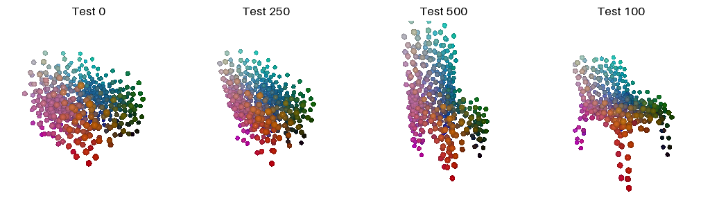
The decoder always produces point i from the same output units. Coloring each index by its mean position over the test set shows a consistent template: the same color lands on the same part of every chair (cyan at the top of the backrest, red at the bottom of the legs, magenta and green on the two sides).
3.1 Implicit Network (10 points)
An MLP maps the image feature and a query point \((x, y, z) \in [-1, 1]^3\) to an occupancy logit. As in Occupancy Networks, the projected feature is added to the projected point, followed by two hidden layers of width 256. Training uses BCE on 8,192 random grid points per image, testing queries the full 32×32×32 meshgrid in (−1, 1)³. 30k steps at lr 4e-4, then 10k at 1e-4. Test F1@0.05: 72.88.
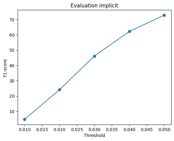
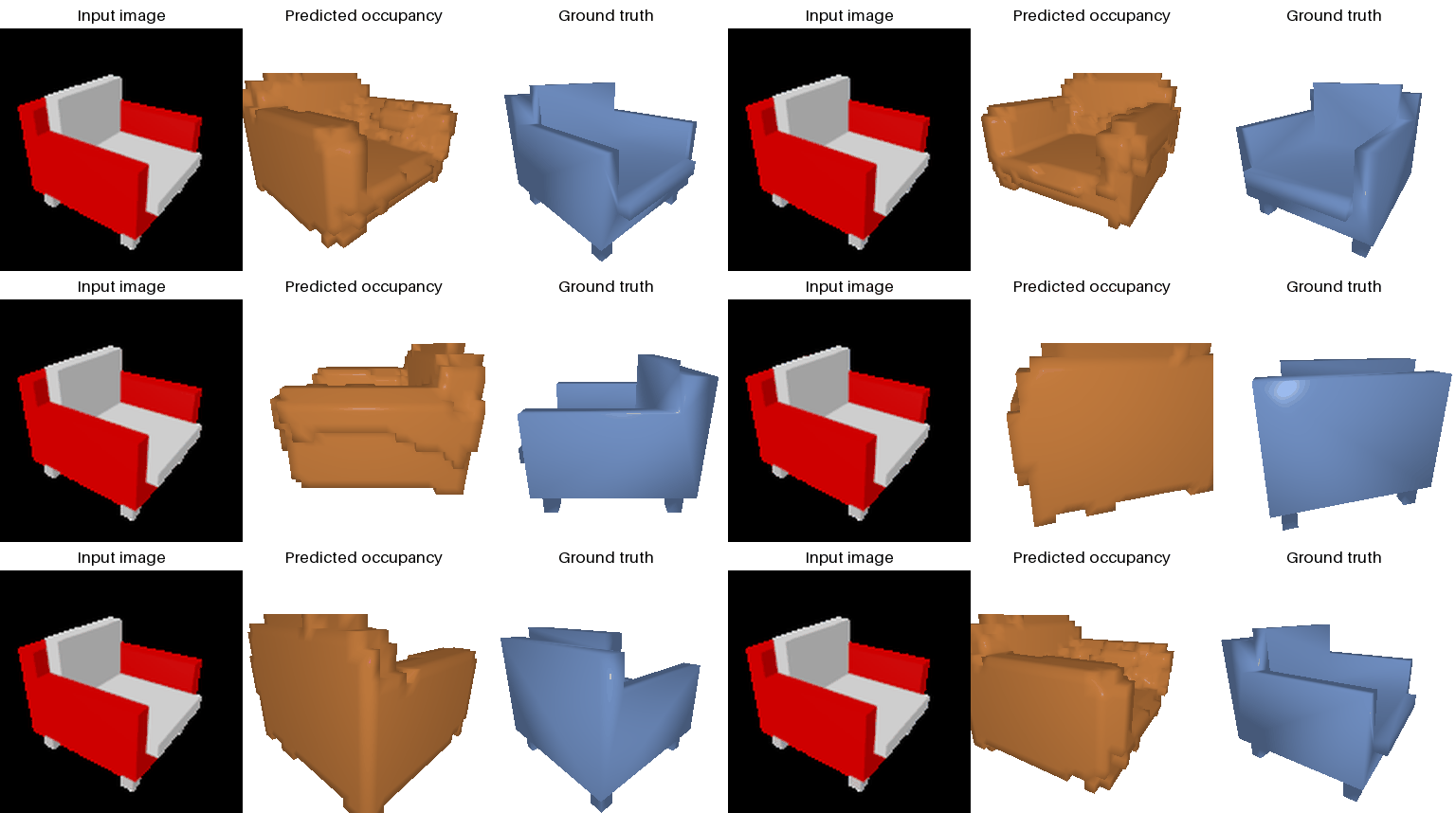
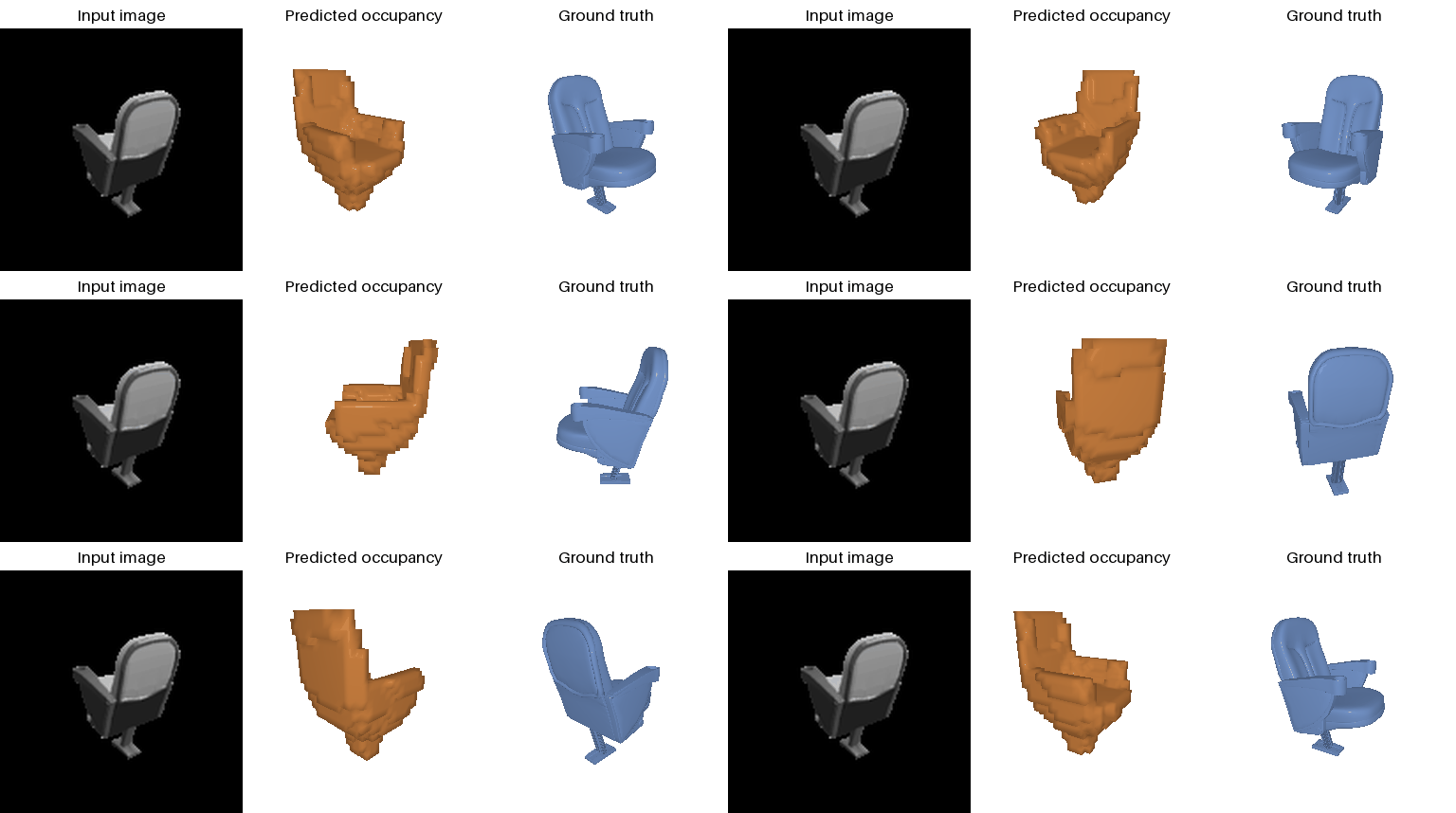
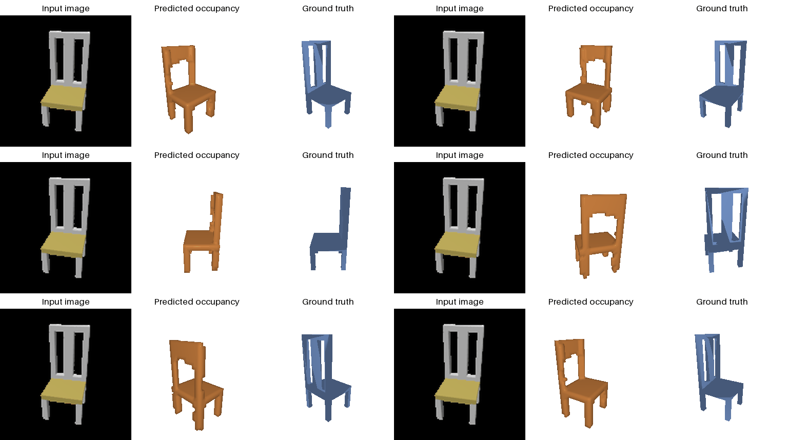
The F1 is close to the voxel decoder's (73.25) with a 0.26M- instead of 11.0M-parameter decoder, and the shapes are cleaner: 1.55 connected pieces per prediction vs. 4.0 for the voxel decoder (ground truth 2.0). Since the network is continuous it can also be queried at 128³, which gives a smooth surface although training only saw the 32³ points.

3.2 Parametric Network (+10 points)
An MLP with the same conditioning maps the image feature and a 2D sample \((u, v) \in [-1, 1]^2\) to a 3D point. Training uses 1,000 random samples per image with Chamfer loss, testing 1,000 fixed Sobol samples. 10k steps, lr 1e-3. Test F1@0.05: 76.36.
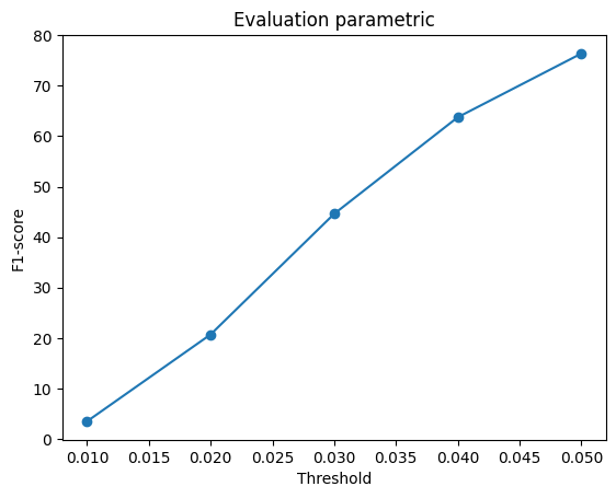


The uv colors land in the same places on every chair: the low-v edge becomes the legs and the high-u, high-v corner the top of the backrest. Mapping a 64×64 uv grid with its triangles shows the learned surface, one sheet folded around the chair. As a single surface it scores between the free point decoder and the mesh (79.76 and 74.25) with a 38× smaller decoder. The boxy armchair (test 0) is its worst case.
