Assignment 2
Geethika Hemkumar (Andrew ID: ghemkuma)
1. Exploring Loss Functions
1.1 Fitting a voxel grid
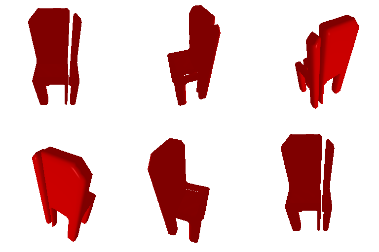
Predicted Voxel Grid (rendered as mesh)

Ground Truth Voxel Grid (rendered as mesh)
1.2 Fitting a point cloud
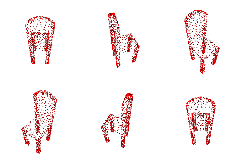
Predicted Point Cloud

Ground Truth Point Cloud
1.3 Fitting a mesh
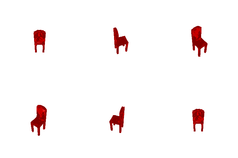
Predicted Mesh

Ground Truth Mesh
2. Reconstructing 3D from single view
2.1 Image to voxel grid
Examples
Image
Ground Truth
Prediction
Example 1: F1@0.05 of 86.977


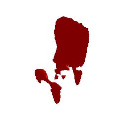
Example 2: F1@0.05 of 96.339


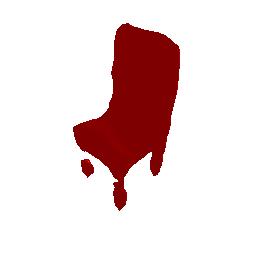
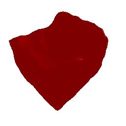
Example 3: F1@0.05 of 44.615


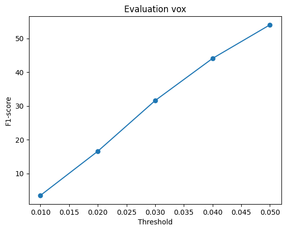
F1 Plot and Average F1@0.05
The F1 plot for image to voxel rendering is below. The average F1@0.05 score across all examples is 54.033.
2.2 Image to point cloud
Examples
Image
Ground Truth
Prediction
Example 1: F1@0.05 of 87.387


Example 2: F1@0.05 of 39.749


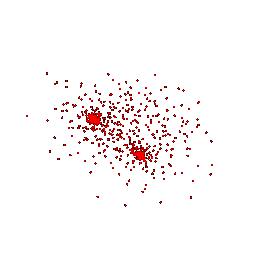
Example 3: F1@0.05 of 68.558


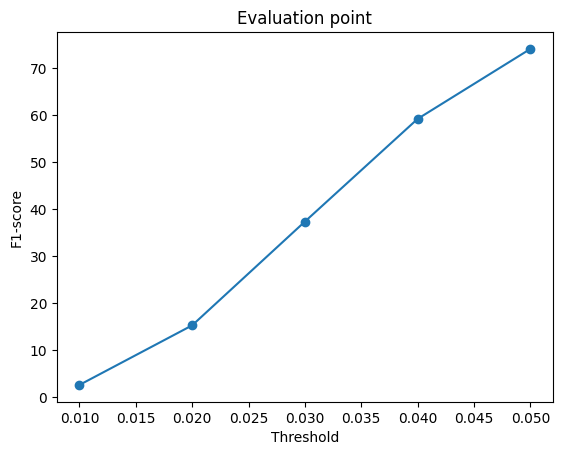
F1 Plot and Average F1@0.05
The F1 plot for image to point cloud rendering is below. The average F1@0.05 score across all examples is 74.166.
2.3 Image to mesh
Examples
Image
Ground Truth
Prediction
Example 1: F1@0.05 of 72.887


Example 2: F1@0.05 of 82.318


Example 3: F1@0.05 of 47.858


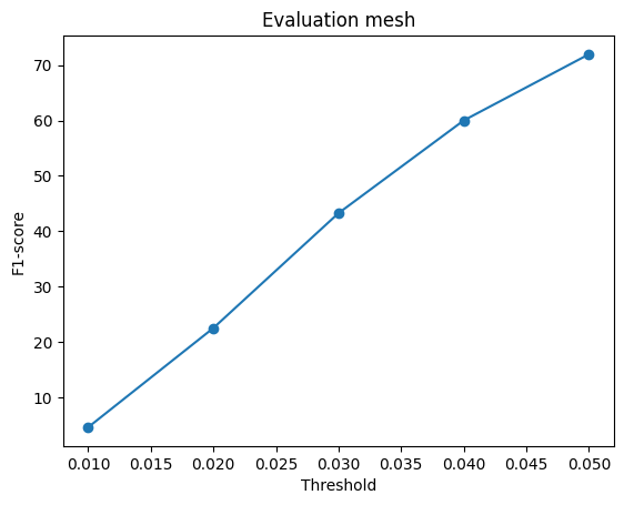
F1 Plot and Average F1@0.05
The F1 plot for image to mesh rendering, initialized with a level 4 ico_sphere, is below. The average F1@0.05 score across all examples is 71.947.
Quantitative Comparison of Meshes vs Pointclouds vs Voxel Grids
| Voxel Grid | Point Cloud | Mesh initialized with sphere | Mesh initialized with cube | |
|---|---|---|---|---|
| Average F1@0.05 evaluation score | 54.033 | 74.166 | 71.947 | 71.507 |
| Iterations trained | 54k | 4k | 10k | 10k |
The above table compares the average F1@0.05 scores for 3D reconstruction across representations. The number of iterations each model was trained for is also included for context.
The order of performance, from worst to best is:
- Image to voxel grid
- Image to mesh (both variations)
- Image to point cloud
The prediction space of a voxel grid is much higher compared to point clouds and meshes (3D for voxel grids vs 2D for point clouds / meshes). Intuitively, this would lead to needing a lot more data / iterations to achieve a higher average performance compared to the 2D representations.
The prediction space of point clouds and meshes are both 2D (the dimension is $(N,3)$, where N is the number of points/vertices). The key difference between point clouds and meshes is that point clouds do not encode connectivity between points. This makes point cloud prediction comparatively easier, which intuitively can explain why the image to point cloud model can achieve a higher performance in less iterations compared to the image to mesh models.
2.4 Analyse effects of hyperparams variations
I chose to change the initial mesh used for image to mesh prediction to a cube centered at the origin. I created a simple cube mesh (8 vertices, 12 faces) and subdivided its faces 4 times, leading to $12*4^4=3072$ faces.
Examples
The same 3 test samples used in Question 2.3 are shown below. The reported F1@0.05 scores in each row header are for the evaluations with the mesh prediction model initialized with a cube mesh.
For comparison, the predicted mesh from the model initialized with the ico_sphere is shown in the fourth column. Please see the row headers of Question 2.3 for the corresponding F1@0.05 scores.
Image
Ground Truth
Prediction (init with cube mesh)
Prediction (init with sphere mesh)
Example 1: F1@0.05 of 83.306


Example 2: F1@0.05 of 84.124


Example 3: F1@0.05 of 55.215


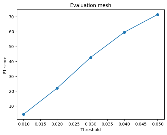
F1 Plot and Average F1@0.05
The F1 plot for image to mesh rendering, initialized with the cube mesh mentioned above, is below. The average F1@0.05 score across all examples is 71.507.
Analysis of Hyperparameter Variation
Qualitatively, the general shapes of the predicted meshes are similar for both models across the three examples shown above. There is some variation in smoothness of the predicted mesh across the chosen examples (the model initialized with the sphere mesh produced a smoother mesh for the first and third examples, while the model initialized with the cube mesh produced a smoother mesh for the second example).
| F1@0.05 scores | Example 1 | Example 2 | Example 3 | Average |
|---|---|---|---|---|
| Sphere | 72.887 | 82.318 | 47.858 | 71.947 |
| Cube | 83.806 | 84.124 | 55.215 | 71.507 |
The above table compares the performance of the two models. The average F1@0.05 score across all evaluation samples is very similar for the model initialized with a sphere mesh (F1@0.05 of 71.947) and the model initialized with a cube mesh (F1@0.05 of 71.507), with the sphere mesh initialized model having a slightly higher average F1@0.05 score.
The sphere mesh model performs worse for all three examples, but both models perform similarly for the second example. A possible intuition for why is that the first and third examples have a structure that is more similar to a cube/rectangular prism, so less deformation is needed from a cube mesh compared to a sphere. The second example has two protruding legs in the back, which requires more deformation for both shapes.
2.5 Interpret your model
To gain some intuition on what the voxel, point cloud, and mesh prediction models are learning, I decided to understand how much various levels of Gaussian blue would affect the models' predictions. I used the following four levels of blur:
- None: no blur applied to the image
- Low: Gaussian blur with kernel_size of 3, sigma of 1.0
- Medium (med): Gaussian blur with kernel_size of 7, sigma of 3.0
- High (hi): Gaussian blur with kernel_size of 11, sigma of 5.0
Below are the predictions for the three models (voxel, point, and mesh prediction) for one example in the dataset (110) with the above levels of blur (the gifs on the right cycle through these levels).
Adding more blur reduces the amount of detail that is apparent in the input image. This causes the resulting predictions to lose some of the example-specific structure, showing that the model is able to understand chair-specific properties to some level.
Ground Truth
Input image (left) and prediction (right) at different blur levels
Voxel


Point


Mesh


Quantitative Evaluation
Evaluation plots (updated to show the F1 scores at various thresholds for each blur level) for the voxel, point, and mesh models are below.
The amount of blurring has the least affect on point cloud prediction, as the F1 scores are very similar across blur levels. This indicates that point cloud prediction does not rely as much on fine-grained details in the image.
Interestingly, blurring helps the F1 score of voxel prediction, which may indicate that the model is not capturing chair-specific details properly when predicting voxel grids.
For mesh prediction, low levels of blurring helps but medium/high levels harm the performance, indicating that mesh deformation prediction is comparatively more sensitive to loss of detail in the input image.


