16‑825 · Learning for 3D Vision · Assignment 2
Single-View to 3D
1 · Exploring Loss Functions
Fitting a single shape directly
1.1 · 4 pts, 1.2 · 3 pts, 1.3 · 3 pts
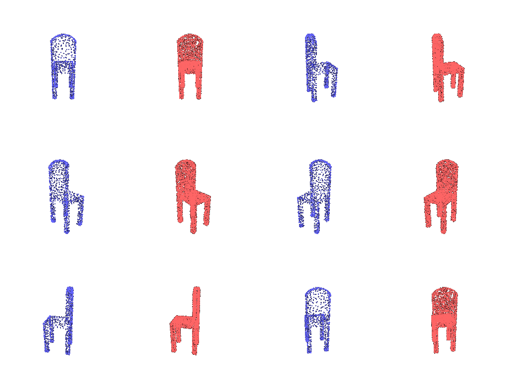
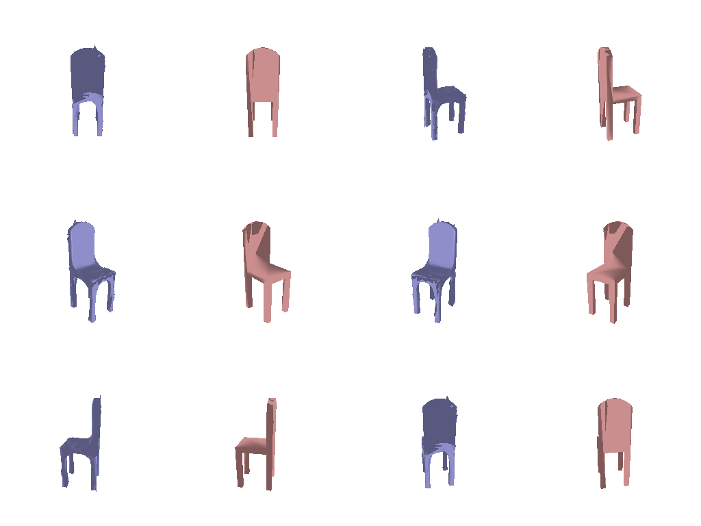
Here there is no network: the source shape itself is optimized with Adam until it matches one target chair. Each gif shows the fitted source (left, blue) next to the target (right, pink), rendered with the turntable tools from Assignment 1.
1.1 Voxel grid: binary cross-entropy
The 32³ source grid is unconstrained, so it is treated as logits and compared to the 0/1 target with binary_cross_entropy_with_logits, which applies the sigmoid inside the loss for numerical stability. After 10,000 steps the loss falls from 0.97 to 0.07. For rendering, the grid goes through a sigmoid, then marching cubes at 0.5, then a map from cell indices back to world coordinates (the dataset stores the grid in [Z, Y, X] order).

.binvox points to the mesh's bounding box per axis, so one slice receives no points after rounding.1.2 Point cloud: chamfer loss
Implemented from scratch with knn_points (K = 1): the mean squared distance from every source point to its nearest target point, plus the same from target to source. The first term pulls points onto the surface, and the second makes sure every part of the surface gets covered. 5,000 points, 20,000 steps.
1.3 Mesh: chamfer + Laplacian smoothing
An ico_sphere(4) is deformed by learned per-vertex offsets. The loss is chamfer on 5,000 points sampled from each surface plus 0.1 × uniform Laplacian smoothing (mesh_laplacian_smoothing), which penalizes each vertex for sitting far from the average of its neighbours, so spikes get pulled back in. 10,000 steps.
2.1 · Image to Voxel Grid
Image → 32³ occupancy
20 pts
Training setup (all of Q2): ResNet18 encoder (ImageNet-pretrained, fine-tuned end to end) → 512-d feature → type-specific decoder. 10,000 iterations, batch size 32, Adam, lr 4×10⁻⁴. The checkpoint from step 9,000 is evaluated on all 678 test chairs.
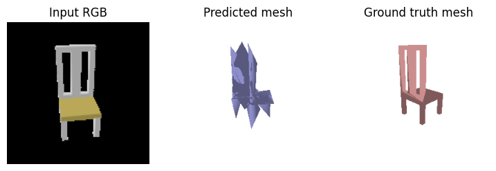
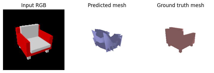
Decoder: Linear 512 → 128×4³, then three 3D transposed convolutions (4³ → 8³ → 16³ → 32³, each followed by BatchNorm and ReLU), then a final convolution to one occupancy logit per voxel. Trained with BCE-with-logits. At evaluation the logits pass through a sigmoid and a mesh is extracted with marching cubes at an occupancy threshold of 0.3. I tuned this threshold down from the default 0.5 because the model is under-confident on thin parts (see 2.4).
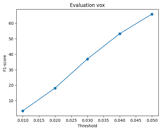
eval_vox.png).Three test examples with full coverage, chosen from the chairs with the highest F1 (input RGB | predicted voxels | ground-truth mesh), with each chair's own F1@0.05:
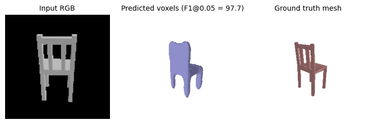
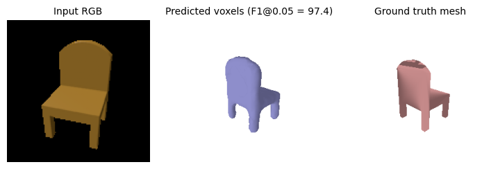
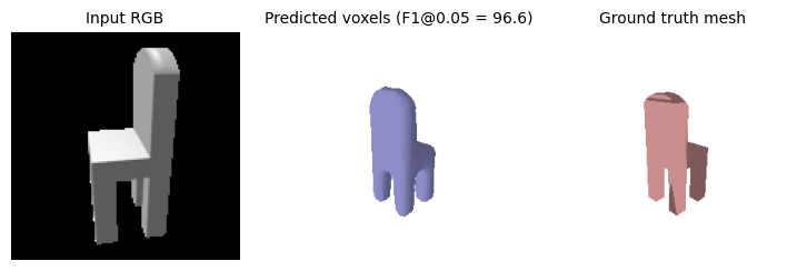
The model reliably recovers large solid parts (backrest, seat) and loses thin ones (legs, arms, slats). Two causes: resolution, since one cell is about 3% of the chair, and class imbalance, since about 96% of voxels are empty, so BCE rewards predicting "empty" whenever the model is unsure. At the default 0.5 threshold this left thin parts out entirely, and about 5% of test images had no voxel above 0.5 at all. At 0.3 only 3 of the 678 test predictions are empty. Empty predictions are scored F1 = 0. (I added this check to evaluate(), which otherwise crashes on an empty mesh.)
2.2 · Image to Point Cloud
Image → 1,000 points
20 pts
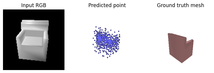
Decoder: an MLP 512 → 1024 → 2048 → 1000×3 (ReLU between layers, no output activation, since coordinates can be negative), reshaped to 1,000 points and trained with the chamfer loss from 1.2. A fully connected decoder fits here because a point cloud has no grid: output index i has no spatial neighbours, so convolutions would impose a structure that doesn't exist.
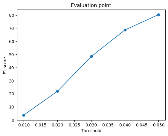
eval_point.png).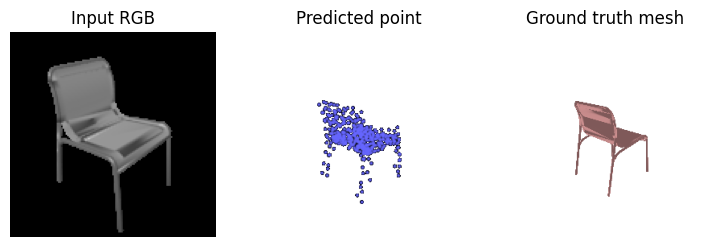
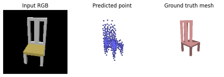
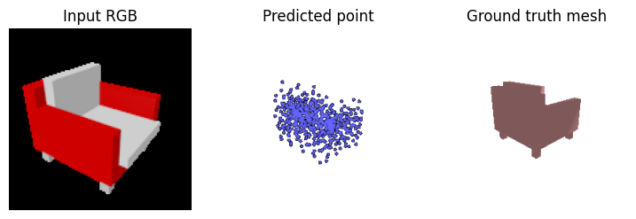
Free-floating points have no resolution limit and no threshold that can delete uncertain parts, so thin structures survive. The cost is noise: scattered outliers, and uneven density with clusters in some places and gaps in others (see 2.5).
2.3 · Image to Mesh
Image → deformed sphere
20 pts
Decoder: an MLP 512 → 1024 → 2048 → 2562×3 that predicts an offset for every vertex of ico_sphere(4). Trained with chamfer (1,000 points sampled from each mesh) plus 0.1 × Laplacian smoothing, the same losses as 1.3.
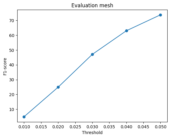
eval_mesh.png).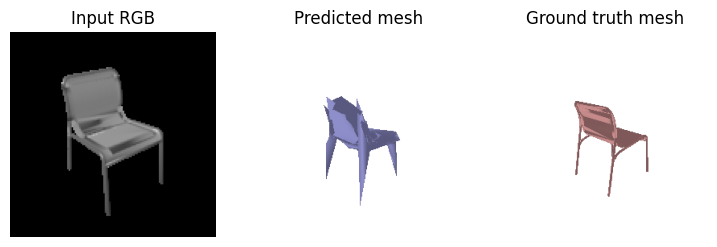
Voxels vs points vs mesh
| Representation | F1@0.05 |
|---|---|
| Voxels (2.1, threshold 0.3) | 65.88 |
| Point cloud (2.2) | 80.38 |
| Mesh (2.3) | 73.77 |
Points score highest because each point moves independently, with no resolution limit, no connectivity constraint and no threshold. F1 is also measured on points, which matches this output directly. Meshes come second: they also have no resolution limit and can form thin legs, but they must stay one connected deformed sphere. A sphere cannot open holes (between legs, between slats), so it stretches and folds across them, and those spikes and stretched triangles put sampled points in the wrong places. The smoothing term trades some accuracy for a tidier surface. Voxels score lowest: at 32³ thin parts are thinner than a cell, and the under-confident model gives them low occupancy. Lowering the threshold to 0.3 recovers much of this (54 → 66), but only partly. Even the ground-truth voxels score only about 78 against the mesh (measured on 100 test chairs), because of resolution and the loader's distorted voxelization. So 66 is about 85% of what any voxel output could reach under this evaluation.
2.4 · Hyperparameter Analysis
The voxel occupancy threshold
10 pts
2.1 suggested the voxel model is under-confident: thin parts get occupancy probabilities around 0.3–0.4, below the default marching-cubes level of 0.5. To test this, the same trained model was evaluated with the isovalue set to 0.2, 0.3, 0.4 and 0.5. No retraining was needed.
| Threshold | F1@0.05 |
|---|---|
| 0.2 | 57.93 |
| 0.3 (used in 2.1 and 3.1) | 65.88 |
| 0.4 | 62.67 |
| 0.5 (default) | 54.01 |


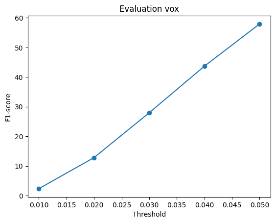
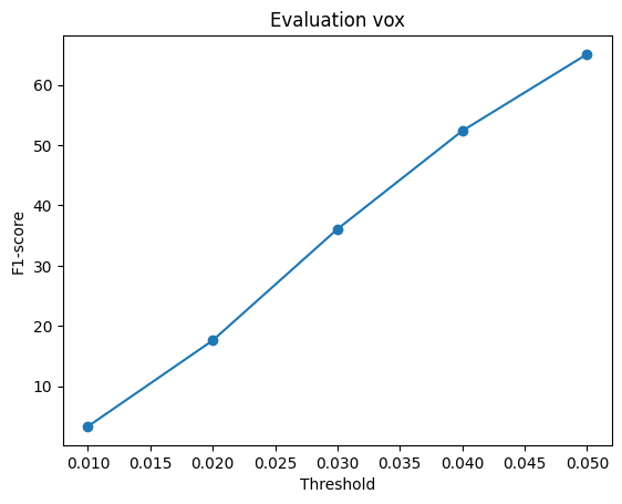
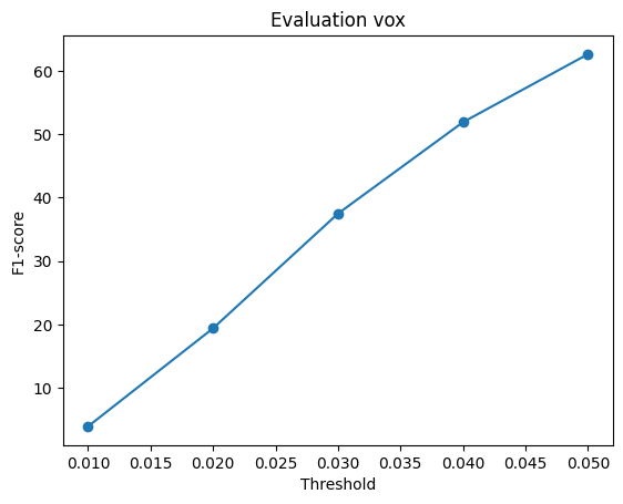
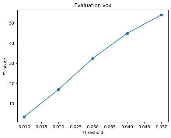
Conclusion. F1 has a clear peak at 0.3, about 11 points above the default. The threshold trades recall (keeping uncertain thin parts) against precision (not counting uncertain empty space as chair). Because 96% of training voxels are empty, BCE pushes uncertain cells toward "empty", so the best cutoff for this model is below 0.5. Going too far (0.2) inflates the shape and F1 drops again. Based on this, 0.3 is used for the voxel results in 2.1 and 3.1. The threshold was chosen on the test set, because the provided split has no validation set, so the 0.3 numbers are slightly optimistic. A weighted BCE (pos_weight) would address the imbalance during training instead of at test time. Note: each evaluation picks a random input view per chair, so repeated runs vary by about ±1 F1 (a second run at 0.3 gave 65.11).
2.5 · Interpreting the Models
Where they fail, and what the point decoder learned
10 pts
Error heatmaps: where each model fails
Each point is coloured by its distance to the nearest point on the other shape (blue = 0, red ≥ 0.05, the F1 threshold). "Prediction error" colours the prediction, which corresponds to precision. "Missed GT parts" colours the true surface by distance to the prediction, which corresponds to recall.
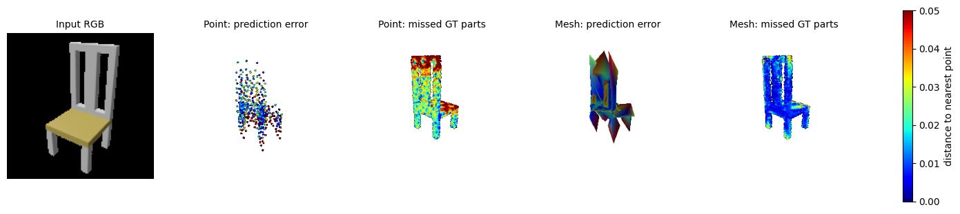
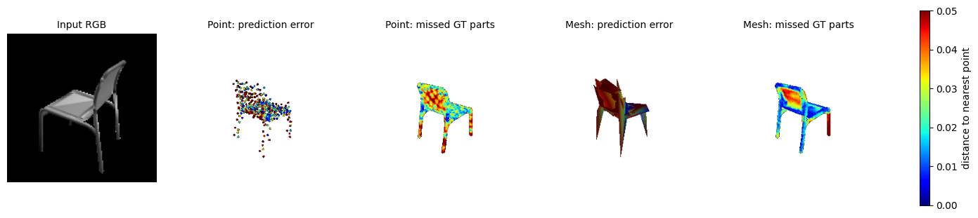
The two models fail in opposite ways. The point model has a blue core with scattered red outliers (precision), and it misses the centres of large flat areas such as the seat and back (recall), because its 1,000 points are spread unevenly. The mesh covers the surface (its recall panels are almost all blue), but its spikes and folds overshoot the chair and show up red in the precision panel.
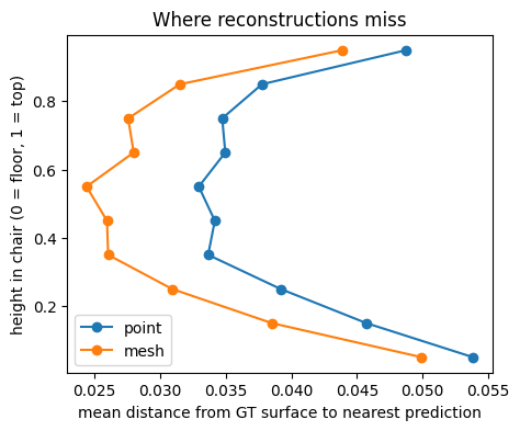
Over 200 chairs both curves are C-shaped: errors are largest at the legs (bottom) and the top of the backrest, and smallest at the seat. The extremities are the thinnest, most varied and most often partly hidden parts. (Compare the curves' shapes, not their levels: the mesh is sampled at 5,000 points and the point model only outputs 1,000.)
Does each output point of the point decoder stick to one part?
Chamfer loss ignores point order, so nothing forces output point #i to mean anything. To test this, every output index is coloured by where it lands in the first chair (x, y, z → r, g, b), and the same colours are reused for other chairs. Idea inspired by AtlasNet / FoldingNet.

The colours land on the same parts in every chair: cyan on the upper backrest, dark blue on the back-left legs, pink on the front legs, orange on the seat's right edge. After scaling each chair to a unit box, an output index moves about 3.3× less between chairs than chance. So the MLP has learned an implicit template: each output slot specializes in one region, and the network deforms that template per chair. This also explains the uneven density above, since slots are assigned by part rather than spread evenly over the surface area.
3 · Other Architectures / Datasets
Extensions
3.1 Implicit network 10 pts
Decoder: an MLP that answers one question per query, "is 3D point (x, y, z) inside this chair?". The input is the 512-d image feature concatenated with the coordinate (515 numbers), passed through 256 → 256 → 256 → 1 with ReLU, and the output is one occupancy logit, as in Occupancy Networks. During training each chair is queried at 4,096 random points of a 32³ grid in (−1, 1)³ (BCE against the ground-truth voxel at that cell). At test time all 32,768 grid points are queried and reshaped into a voxel grid, so it is evaluated exactly like 2.1, with the same 0.3 threshold.
| Voxel decoder | threshold 0.3 | threshold 0.5 |
|---|---|---|
| 3D transposed convolutions (2.1) | 65.88 | 54.01 |
| Implicit MLP (3.1) | 58.23 | 40.20 |
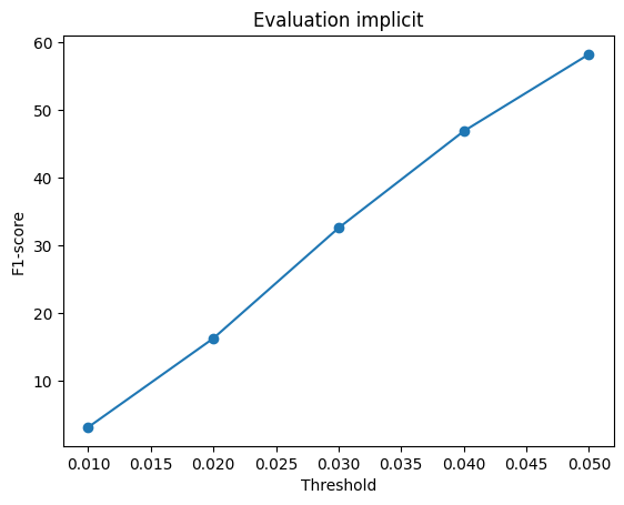
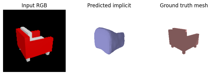

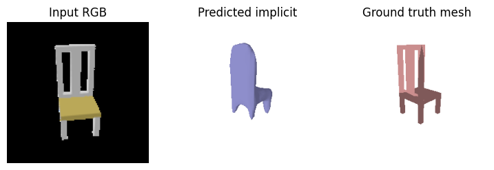
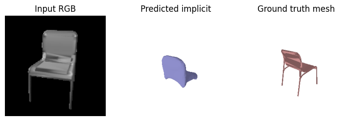
The implicit decoder produces smoother surfaces than the convolutional one, since the shape is a continuous function of the coordinates. But it is less accurate (58 vs 66) and loses thin parts more often. Every query sees only one global 512-d feature plus its coordinates, while 3D convolutions share local spatial structure between neighbouring cells. Uniform random queries are also about 95% empty, so it suffers even more from the class imbalance in 2.4. Lowering the threshold from 0.5 to 0.3 helps it more (+18 F1, and empty predictions fall from 111 to 29 of 678). Its advantage is resolution independence: the same network can be queried on any grid without changing the architecture.
3.2 Parametric network 10 pts
Decoder: a learned function that "folds" a flat square onto the chair's surface, following AtlasNet / FoldingNet. For every shape, 1,000 random 2D samples (u, v) are drawn from [0, 1]². Each one is concatenated with the 512-d image feature (514 numbers) and mapped by a shared MLP 514 → 512 → 256 → 128 → 3 (ReLU, Tanh output) to a 3D point. Trained with the chamfer loss against 1,000 points sampled from the ground-truth mesh, with the same setup as 2.2. Because (u, v) is resampled every step, the network learns a map for the whole square rather than for 1,000 fixed slots, so any number of points can be generated at test time.
| Point-cloud decoder | F1@0.05 |
|---|---|
| MLP to 1,000×3 fixed outputs (2.2) | 80.38 |
| Parametric (u, v) → (x, y, z) (3.2) | 71.54 |
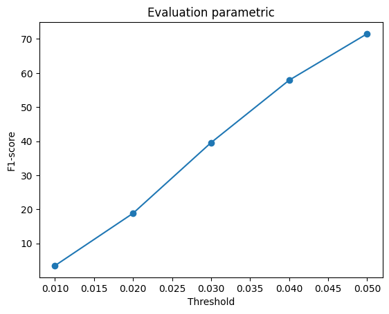
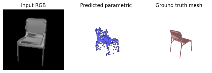
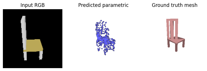
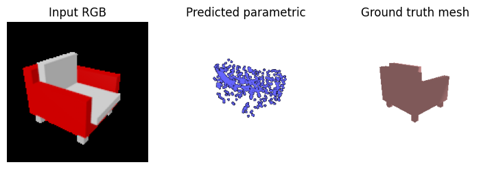
The parametric decoder recovers the overall shape but is less precise than the 2.2 decoder (71.5 vs 80.4), with blurrier clouds and weaker legs. Two reasons stand out. One sheet has to cover everything: a single square must be folded onto a chair that has holes and thin separate parts (legs, slats), so parts of the sheet get stretched across gaps, which puts points in empty space. AtlasNet uses several patches for exactly this reason. Capacity is shared: in 2.2 every output slot has its own weights in the last layer (about 6M parameters), so a slot can specialize in one leg, as 2.5 showed. Here one small MLP must produce every point from (u, v) alone. In exchange, the output is a continuous surface parameterization of any density, rather than a fixed-size, unordered set.
3.3 Extended dataset 10 pts
Setup: the 2.2 point-cloud model (same architecture, 10,000 iterations, batch size 32, lr 4×10⁻⁴) was retrained on the extended split split_3c.json: 3,640 planes, 3,146 cars and 6,100 chairs (12,886 shapes). Both models were then evaluated on the 3-class test set and on the chair test set. Engineering note: car meshes are very large, so loading and sampling the full mesh for every training item made 3-class training about 4× slower and ran out of memory. I therefore sampled 10,000 surface points per training shape once (precompute_points.py), and training draws a fresh random 1,000 of them each step. All evaluation still samples from the real meshes.
| Trained on | Chair test set | 3-class test: airplane | car | chair | all |
|---|---|---|---|---|---|
| Chairs only (2.2) | 80.38 | 65.37 | 68.21 | 80.06 | 72.93 |
| Chairs + cars + planes | 79.36 | 95.90 | 91.58 | 79.27 | 87.04 |
All values are F1@0.05. The "3-class test" columns are the mean F1 per class on split_3c.json's test set (403 planes, 367 cars, 678 chairs). Each evaluation picks a random input view per shape, so repeated runs vary by about ±1.
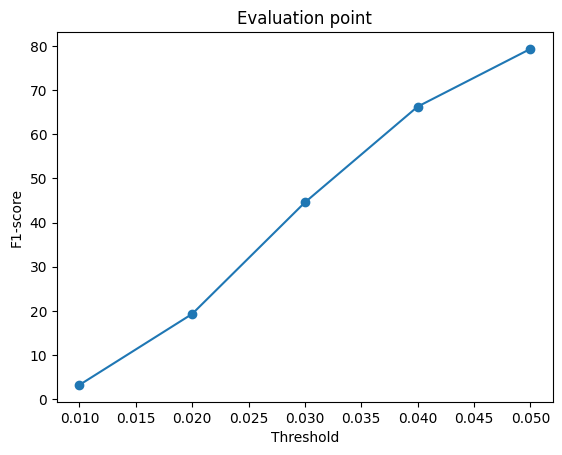
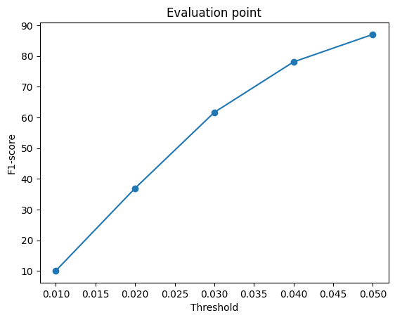
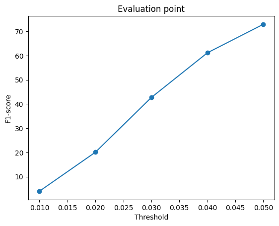
Same test shapes, chair-only model (left column) vs 3-class model (right column):
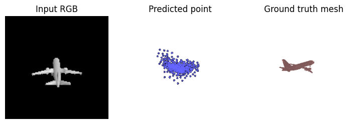
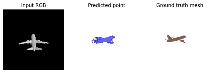
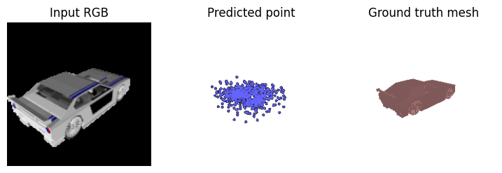
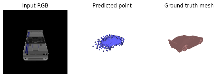

On the same chair test samples, the F1 barely changes (80.4 → 79.4 on the chair split, 80.1 → 79.3 on the chairs of the 3-class split). That is within run-to-run noise, even though chairs are now only 47% of the training data and the network shares its capacity with two other categories. Adding cars and planes neither clearly helps nor clearly hurts chair reconstruction.
On new categories the difference is large. The chair-only model scores only 65–68 on planes and cars, and its outputs show why: whatever the input, it produces a chair-shaped blob. This is the learned per-slot chair template from 2.5 at work. Its outputs have low diversity, so the model behaves more like it is recalling "a chair" than reconstructing the image (as argued by Tatarchenko et al., 2019). The 3-class model instead produces category-appropriate shapes (fuselage and wings, a low car body), so its output diversity follows the input. Planes and cars even score higher than chairs (96 and 92 vs 79). Within each category their shapes are more consistent (every plane has a fuselage and wings in roughly the same layout, every car is a box-like body), whereas chairs vary much more in topology and have thin legs, slats and holes.