Overview and training
This assignment learns directly from unordered point clouds. The baseline PointNet models use shared pointwise features and symmetric maximum pooling for object classification and chair-part segmentation. Two robustness experiments probe rotation and input sparsity, followed by a local-neighborhood architecture for both tasks.
Shared experimental settings
All four trained models use Adam at learning rate 0.001 and 250 epochs. Classification uses batch size 32 and segmentation uses 8. Models are evaluated on the same supplied test splits, without test-time voting. The local and baseline architectures use all 10,000 points during training and standard evaluation.


Q1. Classification
Implementation and training
The classifier applies shared pointwise layers (3 → 64 → 128 → 1024), each with batch normalization and ReLU. Symmetric maximum pooling aggregates the point features into a permutation-invariant object descriptor. Fully connected layers (1024 → 512 → 256 → 3), with layer normalization, ReLU, and dropout, predict class logits. Softmax converts these logits into probabilities during reporting; cross-entropy training uses the logits directly. No transformation blocks are used.
Training used Adam, learning rate 0.001, batch size 32, 10,000 points per object, and 250 epochs. Following the provided training script, the saved checkpoint is selected by the highest test accuracy observed during training, so the test set also serves as the checkpoint-selection set. This is not an untouched final holdout. The best accuracy was first reached at zero-based epoch 182 (epoch 183 when counting from one).
Test result
Accuracy: 97.3767% (928 / 953 objects).
| Ground-truth class | Correct / total | Accuracy |
|---|---|---|
| Chair | 616 / 617 | 99.84% |
| Vase | 86 / 102 | 84.31% |
| Lamp | 226 / 234 | 96.58% |
Confusion matrix (rows: ground truth; columns: predicted chair, vase, lamp):
          chair  vase  lamp
chair       616     0     1
vase          0    86    16
lamp          0     8   226
Random test examples

Six objects were sampled uniformly without replacement with seed 825, independently of prediction correctness. Each panel shows the test index, true class, predicted class, and softmax confidence. Classification uses all 10,000 points; figures draw every fifth point for readability. Colors indicate the plotted z coordinate.
Failure examples and interpretation
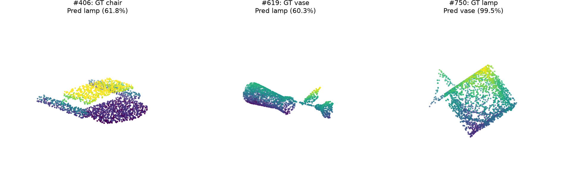
- Chair #406 → lamp (61.8% confidence). Its low, flattened silhouette has little clearly separated backrest structure in this view. Atypical chair geometry may produce global shape features similar to a broad lamp fixture. This is a visual hypothesis rather than a measured attribution of the model's decision.
- Vase #619 → lamp (60.3%). The point cloud has a long narrow body and separated, protruding clusters, rather than a simple compact vessel silhouette. Those features could resemble a lamp stem and attachments; the relatively low confidence is consistent with ambiguity between these two classes.
- Lamp #750 → vase (99.5%). This example has a broad, hollow-looking geometric outline with no clearly isolated thin stem in the rendered view. Its silhouette could resemble a vessel or container. The confident error illustrates that softmax confidence does not guarantee correctness on unusual shapes.
Vase–lamp confusion accounts for 24 of the 25 errors. Their overlapping geometric forms and the absence of appearance cues may contribute. PointNet's independent point processing and global maximum pooling also do not explicitly model local surface neighborhoods, which may make thin parts and openings difficult to distinguish. These are plausible explanations, not experimentally isolated causes.
Reproduce
From the assignment root:
source .venv/bin/activate
python train.py --task cls
python eval_cls.py
python report_q1.py
report_q1.py saves figures, metrics.json, and per-object labels, predictions,
and probabilities in predictions.npz. The results can be incorporated into the
assignment website using the supplied figures and explanations.
Q2. Segmentation
Model and training
The segmentation model accepts (B, N, 3) coordinates and predicts (B, N, 6)
class logits. Shared pointwise layers first produce 64-dimensional local features.
A second stack produces 1024-dimensional features, which are max-pooled over the
points to form an object-level descriptor. That descriptor is broadcast to every
point, concatenated with its local feature, and processed by shared layers
1088 → 512 → 256 → 128 → 6. Batch normalization and ReLU follow hidden layers.
No transformation blocks are used. Cross-entropy consumes logits directly;
softmax can convert logits into probabilities, and argmax selects the part label.
Training used 4,489 chairs, 10,000 points per object, Adam with learning rate 0.001, batch size 8, and 250 epochs. Batch size was reduced from the starter's 32 to accommodate dense feature maps. The provided checkpoint-selection protocol uses test accuracy each epoch: consequently this test split also selects the best checkpoint and is not an untouched holdout. Best accuracy was first reached at epoch 232 (counting from one); the last epoch reached 89.63%.
Overall test accuracy
90.2338% point accuracy across all 617 test chairs and 6,170,000 points. Accuracy is the number of correctly labeled points divided by the total number of points. Because every chair contains the same number of points, it also equals the mean per-object accuracy.
Five GT/prediction comparisons
The first three objects were sampled with seed 825 from the test set, excluding the two lowest-accuracy objects. The last two were deliberately selected as bad predictions. Each static plot draws every third point for readability; reported accuracies use all 10,000 points. Colors consistently denote numeric labels: 0 gray, 1 magenta, 2 cyan, 3 yellow, 4 blue, and 5 red. The README does not define semantic names for the six numeric part IDs, so none are inferred here.
| Object | Selection | Point accuracy | Ground truth GIF | Prediction GIF |
|---|---|---|---|---|
| #102 | Random | 96.64% | GT | Prediction |
| #120 | Random | 96.86% | GT | Prediction |
| #233 | Random | 95.32% | GT | Prediction |
| #235 | Lowest accuracy | 44.19% | GT | Prediction |
| #61 | Second-lowest accuracy | 46.53% | GT | Prediction |
Chair #102 — 96.64%

The model recovers the large cyan, red, and blue regions closely. Remaining mistakes appear mainly around transitions and thin structures. Distinct geometry and a familiar arrangement of parts likely make this object relatively easy.
Chair #120 — 96.86%

The cyan region, red central region, and blue branching support structure are well separated in the prediction. Small discrepancies remain where the thin supports meet the central region. Global context plus per-point geometry is sufficient to recover most of this object's structure.
Chair #233 — 95.32%

The main red, cyan, and blue regions are recognized correctly, including most of the curved blue structure. The prediction loses a few cyan points within the central red region. Small interleaved or adjoining regions are harder to resolve than the broad part boundaries.
Chair #235 — 44.19% (bad prediction)

This broad, dense object has overlapping yellow and red ground-truth regions in the displayed projection. The prediction assigns many points in the upper and left regions to blue or red rather than yellow. The failure is consistent with difficulty distinguishing adjacent surfaces on an atypical shape; explicit local neighborhood features might help, although this experiment does not test that hypothesis directly.
Chair #61 — 46.53% (bad prediction)

The ground truth contains a substantial yellow region, but the model labels most of the upper structure red. It also introduces magenta predictions across the lower cyan region. These are large region-level mistakes rather than only noisy boundaries, suggesting the learned part layout does not match this object's geometry well.
Interpretation and limitations
High aggregate accuracy hides variation between objects and part classes. The two difficult examples exhibit substantial whole-region confusion even though random examples exceed 95% accuracy. PointNet combines independent point features with a global pooled descriptor, but has no explicit local surface-neighborhood reasoning. This is a plausible limitation for neighboring parts of similar shape, not a demonstrated causal explanation. The saved confusion matrix also permits inspection of rare classes that overall point accuracy can underweight.
The GIFs rotate the same point clouds with consistent label colors and allow inspection beyond the single static view. Geometry is unchanged during plotting.
Reproduce
Run from the assignment root:
source .venv/bin/activate
python train.py --task seg --batch_size 8 --num_epochs 250
python report_q2.py
To evaluate and render one chosen object with the standard evaluation entry point:
python eval_seg.py --i 235 --exp_name chair235
metrics.json contains the overall result, confusion matrix, and selected-object
accuracies. predictions.npz contains every test point's prediction and label,
plus per-object accuracies. Figures and text here are ready to incorporate into
the assignment website.
Rotating ground-truth and prediction comparisons
Open an object to compare its labels from multiple viewing directions. Gray, magenta, cyan, yellow, blue, and red represent IDs 0–5.
Chair #102 · 96.64% · random


Chair #120 · 96.86% · random


Chair #233 · 95.32% · random


Chair #235 · 44.19% · lowest accuracy


Chair #61 · 46.53% · lowest accuracy


Q3. Robustness analysis
Two experiments were performed on both the trained Q1 classifier and Q2 segmenter. Checkpoints were fixed; neither model was retrained or fine-tuned. All 953 classification objects and all 617 segmentation objects were evaluated. The baseline reproduces Q1's 97.3767% object accuracy and Q2's 90.2338% point accuracy.

Experiment 1: rotation
Procedure
Rotate every test cloud about the y-axis through the coordinate origin by 0°, 30°, 60°, 90°, or 180°. All 10,000 points are retained. For column-vector coordinates, the applied matrix is:
R_y(theta) = [[ cos(theta), 0, sin(theta)],
              [          0, 1,          0],
              [-sin(theta), 0, cos(theta)]]
Object labels and per-point part labels stay attached to the same objects/points. This evaluates sensitivity to coordinate orientation, not point-order sensitivity. The axis is explicitly y; it is not assumed to be the dataset's vertical axis.
| Rotation | Classification accuracy | Change from Q1 | Segmentation accuracy | Change from Q2 |
|---|---|---|---|---|
| 0° | 97.38% | — | 90.23% | — |
| 30° | 84.16% | −13.22 pp | 74.31% | −15.93 pp |
| 60° | 59.29% | −38.09 pp | 60.20% | −30.04 pp |
| 90° | 65.06% | −32.32 pp | 46.12% | −44.12 pp |
| 180° | 31.06% | −66.32 pp | 59.08% | −31.15 pp |
Classification visualizations

Each row tracks the same object across conditions. Examples deliberately include chair #183 and the vase/lamp failure cases #619 and #750 from Q1. They illustrate behavior, rather than being an unbiased sample. Chair #183 is correct at baseline and 30°, but becomes a vase at 90° and a lamp at 180°. Conversely, the two Q1 failure objects become correct at 180° even though overall performance collapses. Thus rotation can fix individual errors while harming aggregate accuracy.
Segmentation visualizations


Rows use chairs #102, #120, and #235 from Q2; columns preserve sample identity. Part colors consistently encode numeric IDs 0–5. The GT plots rotate geometry without changing part labels. Predicted colors and per-object accuracies show whether the model preserves the original semantic labels under orientation change.
Interpretation
Both models are strongly orientation-sensitive. Symmetric pooling provides permutation invariance for object classification, but does not provide rotation invariance: changing coordinates changes the learned pointwise features. The segmenter also uses coordinate-dependent local features and an orientation-sensitive global descriptor. Neither training pipeline used rotation augmentation or learned transformation blocks. These design choices are consistent with the observed drop, though the experiment does not isolate their separate contributions.
Accuracy is not monotonic in angle: some rotated shapes resemble familiar coordinate patterns more closely than others. For example, segmentation performs better at 180° than at 90°. This does not establish invariance at either angle. Potential remedies include rotation augmentation or rotation-aware features; their effectiveness would require separate training experiments.
Experiment 2: number of input points
Procedure
Keep the original orientation and evaluate 10,000, 2,048, 1,024, and 256 points per object. Uniform sampling is without replacement, using seed 825. A single random permutation of point indices defines nested subsets (256 is contained in 1,024, which is contained in 2,048), shared across objects. The full baseline uses all original points. Segmentation labels are sampled with exactly the same indices, and accuracy is evaluated on retained points only.
| Points | Classification accuracy | Change from Q1 | Segmentation accuracy | Change from Q2 |
|---|---|---|---|---|
| 10,000 | 97.38% | — | 90.23% | — |
| 2,048 | 96.85% | −0.52 pp | 90.25% | +0.01 pp |
| 1,024 | 97.27% | −0.10 pp | 89.87% | −0.36 pp |
| 256 | 96.43% | −0.94 pp | 85.68% | −4.55 pp |
Classification visualizations
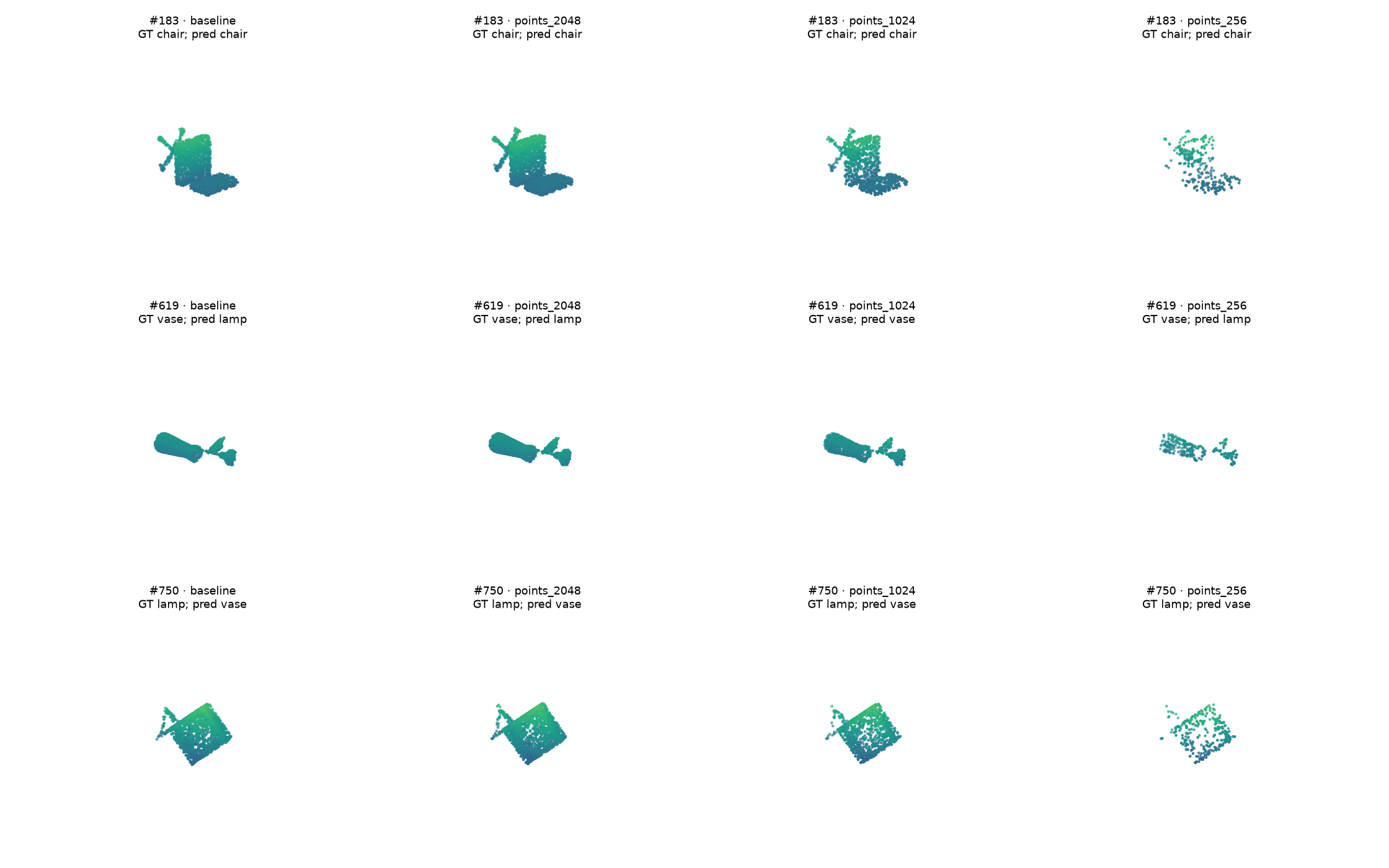
The rows use the same three objects as the rotation experiment. Even with sparse inputs, the broad silhouettes remain visible. Predictions and ground truth are printed in every panel so that sparse-input changes can be compared with Q1.
Segmentation visualizations
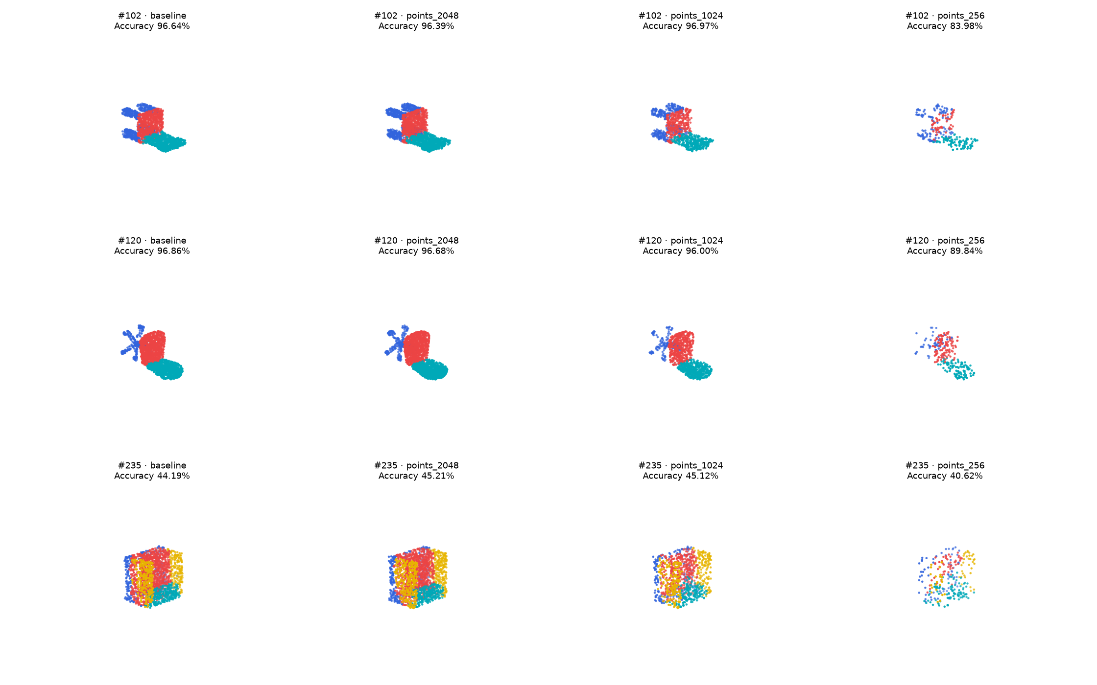

Chair #102 goes from 96.64% at baseline to 83.98% with 256 points; chair #120 falls from 96.86% to 89.84%. The difficult chair #235 remains poor throughout (44.19% at baseline and 40.62% at 256 points). Sparsity removes detail but does not explain all of this object's pre-existing errors.
Interpretation and limitations
Classification is robust to large reductions in point count: 256 points retain 96.43% accuracy, less than one percentage point below baseline. Global max pooling can retain discriminative shape evidence when many redundant surface samples are removed. Segmentation is more sensitive at 256 points, plausibly because thin parts and local boundaries receive less coverage and the pooled context changes.
The tiny segmentation increase at 2,048 points (+0.01 percentage points) should not be interpreted as a meaningful improvement. Each point-count condition uses one sampling seed and evaluates a different set of retained points. Sampling variation and changes in class composition can produce small nonmonotonic changes. Repeated seeds and confidence intervals would strengthen the result. Sparse segmentation accuracy measures labeling of retained points, not reconstruction or labeling of the omitted points.
Reproduction and files
From the assignment root:
.venv/bin/python report_q3.py
metrics.json stores full-precision accuracies, correct counts, denominators,
rotation settings, and point counts for every condition. The script generates all
six qualitative comparison figures and the combined robustness-curve figure.
Static panels draw at most about 2,000 points for clarity; metric computation uses
the complete point set specified for that condition. No test input is augmented
in place or written back to the dataset.
Q4. Bonus: locality
The model uses one local set-abstraction stage inspired by PointNet++. It is not the complete PointNet++ architecture.
128 anchors are selected at evenly spaced ranks along a fixed spatial projection. Each anchor groups its 32 nearest input points. A shared neighborhood encoder processes relative coordinates, absolute anchor coordinates, and learned point features, followed by neighborhood max pooling. Classification pools across anchors; segmentation interpolates the three nearest anchor features with inverse-distance weights and combines these with per-point and global features.
Both models train for 250 epochs with Adam at learning rate 0.001 and all 10,000 input points. Classification uses batch size 32 and segmentation uses 8, matching the respective baselines. Checkpoints are selected by test accuracy, following the starter protocol, so reported test results are not from an untouched holdout. Model capacity and random initialization also differ; changes cannot be attributed solely to locality.
| Task | PointNet | Local | Difference |
|---|---|---|---|
| cls | 97.38% | 97.17% | -0.21 pp |
| seg | 90.23% | 90.36% | +0.13 pp |
Classification comparisons

Rows include a Q1 correct prediction and three Q1 failure cases. Predicted class labels are printed for both models; these fixed examples illustrate changes without selecting only improvements.
Segmentation comparisons

Rows reuse the five Q2 examples, including both low-accuracy objects. Each prediction panel reports its per-object accuracy. Numeric part colors are consistent with Q2.
Interpretation and limitations
Local grouping makes nearby surface geometry available before global pooling, while interpolation passes neighborhood context to dense predictions. This can help distinguish parts that have similar global positions but different nearby structure. It does not guarantee improvement: nearest-neighbor grouping may cross semantic boundaries, fixed anchors may cover thin regions poorly, and a single abstraction stage has a limited spatial hierarchy. Check the measured table and paired examples before attributing gains to this mechanism.
Only one training run per model was used. PointNet and local model parameter counts are stored in metrics.json. Full 10,000-point test clouds are used for both models; static figures subsample only for rendering.
Reproduce with bash run_q4.sh; regenerate this report with .venv/bin/python report_q4.py.
Where locality helped—and where it did not
The two difficult Q2 objects improve: chair #235 rises from 44.19% to 53.19%, and chair #61 from 46.53% to 64.90%. However, chair #120 falls from 96.86% to 95.09%, and #233 from 95.32% to 91.58%; #102 improves slightly to 96.92%. Local context therefore helps some atypical shapes but does not uniformly improve part recognition. These fixed-example comparisons complement the full-test accuracy rather than replacing it.
Reproducibility and scope
All figures and tables are produced from the trained checkpoints and saved experiments. Static figures subsample points only for readability; test metrics use the point count stated in each experiment. GIF rotation changes the viewing direction, while Q3 rotation transforms the actual model input coordinates.
The six segmentation part IDs are shown consistently as gray, magenta, cyan, yellow, blue, and red. The assignment does not provide semantic names for these IDs, so the report uses their numeric labels. Failure explanations describe visible evidence and plausible mechanisms, rather than claiming measured causal attribution.
Generation scripts: report_q1.py, report_q2.py, report_q3.py, and report_q4.py. The webpage is built by build_submission.py.