Two representations, one rendering story.
The first half builds an emission–absorption volume renderer and uses it for inverse rendering, NeRF, hierarchical sampling, and VolSDF. The second half implements the projection, sorting, compositing, training, and view-dependent appearance components of 3D Gaussian splatting.
Implicit fields
Scene properties are queried continuously at sampled 3D positions. Differentiability connects pixel loss back to geometry, density, color, and neural-field parameters.
Explicit Gaussians
A finite collection of oriented 3D Gaussians is projected to screen space and alpha-composited, providing an explicit and efficiently optimizable representation.
Differentiable volume rendering
I implemented the full path from camera pixels to world-space sample points, followed by emission–absorption compositing of color and depth.
Pixels into world-space rays
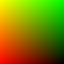
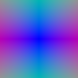
get_pixels_from_image creates an NDC grid in [−1, 1]. get_rays_from_pixels unprojects each point through the camera, subtracts the camera center, and normalizes the resulting direction. The common camera origin is expanded to match the ray batch.
Stratified samples along each ray
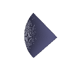
The raysampler linearly spaces depths between the configured near and far planes. Each point is computed as origin + depth × direction; the point and its depth remain paired inside the ray bundle.
Front-to-back emission–absorption
C(r) = Σᵢ wᵢ cᵢ D(r) = Σᵢ wᵢ tᵢ
I compute exclusive transmittance with a shifted cumulative product, then use the same weights to aggregate emitted RGB and sample depths. Chunked evaluation controls memory without changing the rendering equation.

Optimizing an implicit box
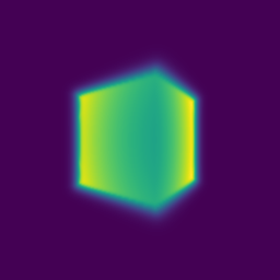
Random ray minibatches make inverse rendering tractable. Image-space supervision recovers the box center and side lengths without direct 3D labels.
Memory-aware sampling
I uniformly sample pixel indices without replacement, convert those selected pixels to NDC coordinates, generate their camera rays, and sample matching ground-truth colors. This reduces each optimization step from a full image to 4,096 informative rays.
Image-space MSE
The predicted RGB for each sampled ray is compared against the corresponding ground-truth pixel with mean squared error. Gradients pass through volume weights and the box SDF to its trainable center and dimensions.
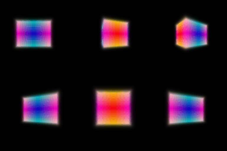
Before optimization




After optimization


Optimizing a NeRF
The analytic volume is replaced with an MLP that learns density and color as continuous functions of 3D position.
Position-encoded neural field
Six-frequency harmonic encoding maps each 3D sample to a high-dimensional basis. A six-layer, 128-unit MLP predicts non-negative density through ReLU and RGB through sigmoid. A skip connection reintroduces the encoded position at layer three to preserve high-frequency information.
Multi-view image supervision
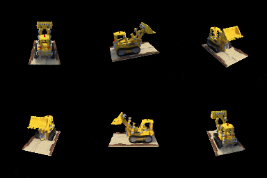
The Lego NeRF trains for 250 epochs at 128² resolution with 1,024 rays per batch, 128 samples per ray, Adam at 5×10⁻⁴, and step decay by 0.8 every 50 epochs. The objective is RGB MSE.
NeRF extras
All three optional extensions were implemented: view-dependent emission, hierarchical coarse/fine sampling, and a learned signed-distance surface with volumetric rendering.
Separating geometry from directional appearance
Density and a learned feature vector come from position alone. A color head combines that feature with a harmonic encoding of the normalized ray direction, allowing specular and direction-dependent appearance without letting viewing direction alter geometry.


Spend samples where matter exists
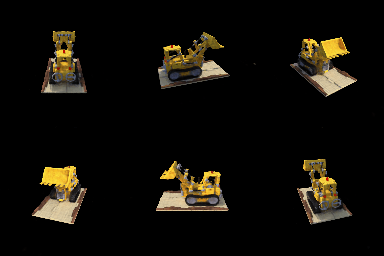
A 64-sample coarse pass estimates ray weights. Inverse-CDF sampling then draws 128 additional depths from this distribution, and the merged depths are sorted for a fine rendering. Compared with uniform 128-sample rendering, this concentrates computation near occupied regions and object boundaries.
A neural surface rendered as density
A six-layer distance MLP predicts signed distance, while a two-layer color head predicts RGB. The Eikonal term encourages unit gradient magnitude, making the learned scalar field behave like an SDF. I used α = 10, β = 0.05, an Eikonal weight of 0.02, 128 samples per ray, and 250 epochs.
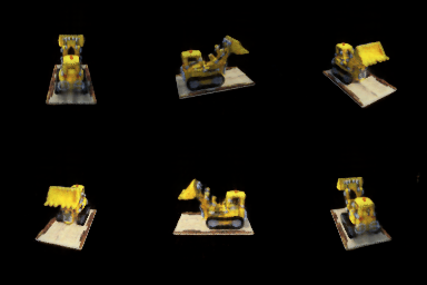
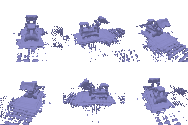
- α controls density scale. Larger α makes occupied regions more opaque and strengthens termination near the surface.
- β controls boundary softness. High β spreads density over a wide band, yielding smoother gradients but a thicker, biased surface. Low β approaches a sharp step around zero level-set.
- Training versus accuracy. High β is easier early in training because gradients act over a wider region. Low β can recover a more precise surface, but optimization becomes more sensitive because useful gradients are concentrated near the surface.
3D Gaussian rasterization
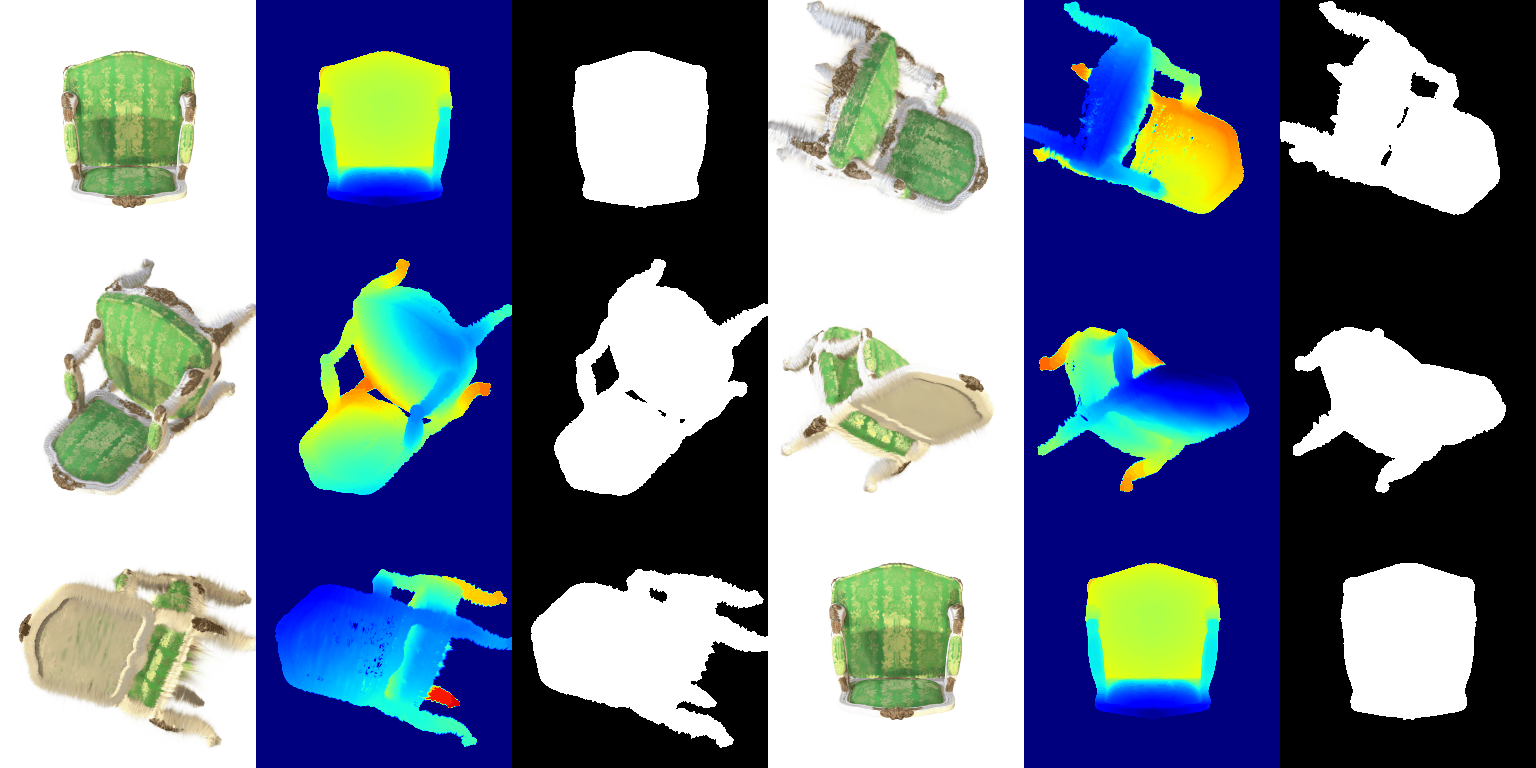
I implemented a vectorized rasterization pipeline that projects oriented 3D Gaussians, evaluates them on pixels, sorts them by depth, and composites color, depth, and silhouettes.
Projection & evaluation
Quaternion rotation and axis scales form each 3D covariance. The camera Jacobian maps it into a stabilized 2D covariance; projected means locate the splats. Pixel power is the vectorized Mahalanobis term −½(x−μ)ᵀΣ⁻¹(x−μ).
Ordering & visibility
Gaussians behind the camera are filtered, and remaining splats are sorted front-to-back by camera-space depth. Opacity times the Gaussian response gives α; an exclusive cumulative product gives transmittance.
Splatting
Color, depth, and mask use the common weight Tα. Mini-batches carry final transmittance forward, preserving global compositing order. Background contributes only through remaining transmittance (1−mask).
Training a Gaussian scene
Starting from a supplied point cloud, I optimized 10,000 isotropic Gaussians to reproduce multi-view images of a toy truck.
| Parameter group | Learning rate | Reasoning |
|---|---|---|
| Opacity logits | 0.05 | Fast visibility adjustment. |
| Log scales | 0.005 | Controlled footprint changes. |
| Colors | 0.0025 | Stable appearance fitting. |
| Means | 0.00016 | Conservative geometric motion. |
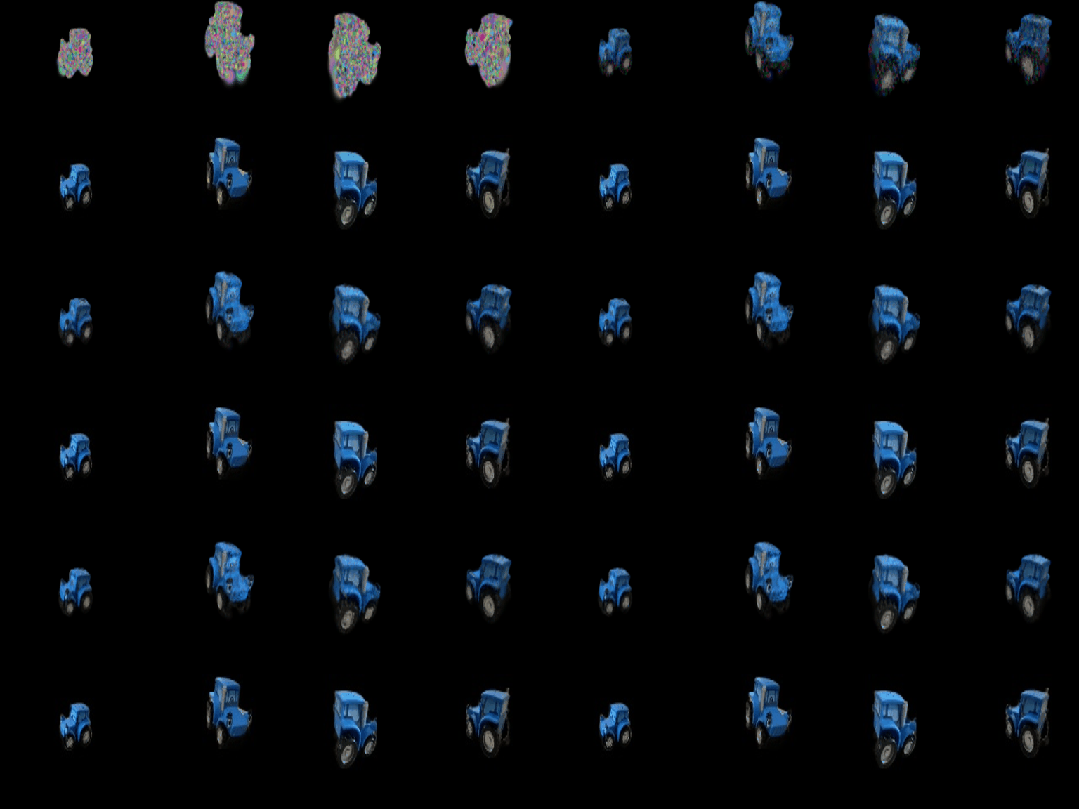

The model learns opacity, scale, color, and means with Adam. Rotations are fixed because rotating an isotropic Gaussian leaves its covariance unchanged. The high held-out scores and stable orbit indicate strong view consistency.
Gaussian extensions
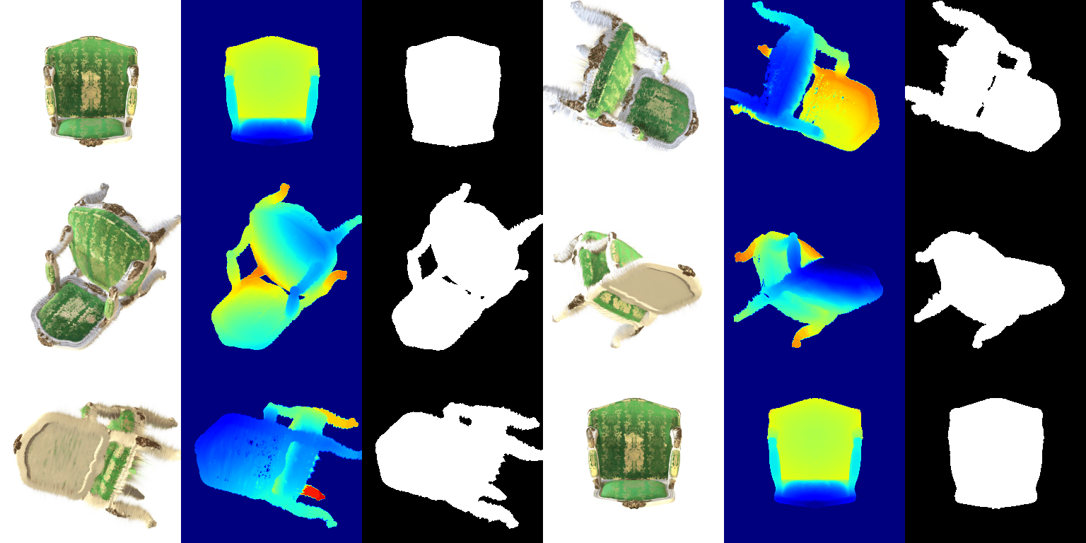
Both extensions were completed: degree-three spherical-harmonic rendering and harder-scene training from random initialization.
View-dependent Gaussian appearance
I evaluate all 16 real SH basis terms through degree three for each RGB channel. Directions are normalized world-space vectors from the camera center to each Gaussian. The original degree-zero path remains available for a controlled comparison.


Random initialization on Materials
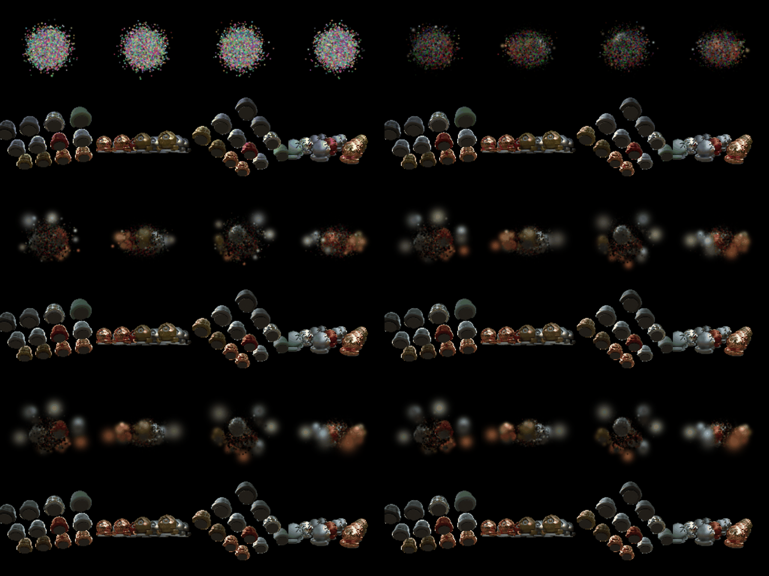
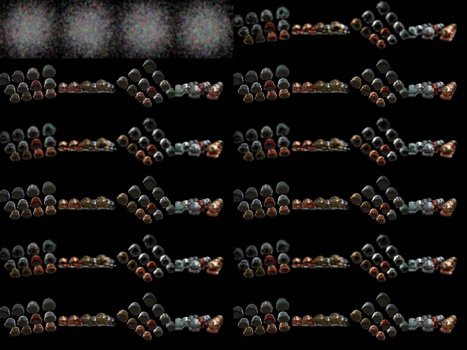
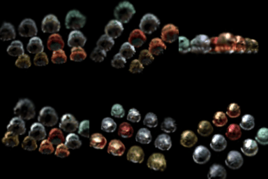
The baseline transfers the Task 6 recipe directly: 10,000 random isotropic Gaussians, L1 loss, and the same learning rates. The improved model targets the failure modes visible in the baseline—poor initial scene coverage, opaque blobs, limited shape flexibility, and blurred structural detail.
| Method | Iterations | Representation | Loss | PSNR | SSIM |
|---|---|---|---|---|---|
| Task 6 baseline | 1,000 | 10k isotropic | L1 | 18.226 dB | 0.651 |
| Improved | 3,000 | 10k anisotropic | 0.8 L1 + 0.2 DSSIM | 22.106 dB | 0.824 |
Improved learning-rate schedule
Each parameter group uses its own initial learning rate and decays exponentially over 3,000 iterations to one tenth of that value.
| Parameter group | Initial learning rate | Final learning rate |
|---|---|---|
| Opacity logits | 0.025 | 0.0025 |
| Log scales | 0.003 | 0.0003 |
| Colors | 0.01 | 0.001 |
| Means | 0.001 | 0.0001 |
| Quaternions | 0.001 | 0.0001 |

Better early gradients
I spread random means over a region three times wider, initialized opacity at 0.1 instead of near one, and set initial scale to 0.03. Wider coverage reduces the chance that scene regions receive no splats; lower opacity prevents early occlusion from saturated blobs.
Anisotropic shape
Three independent scales plus trainable quaternions let Gaussians elongate and rotate along object surfaces. This represents boundaries with fewer primitives than spheres and reduces the soft, circular artifacts visible in the baseline.
L1 + structural similarity
DSSIM adds local luminance, contrast, and structural supervision to per-pixel L1. This directly targets the blurred organization of the baseline and aligns with the large SSIM improvement.
Longer, scheduled training
The improved run uses 3,000 iterations, faster initial color/position learning, quaternion optimization, and exponential decay to one tenth of each initial rate. Large early steps organize the scene; smaller late steps refine it.