Voxel F1@0.05: 75.83
Point cloud F1@0.05: 76.20
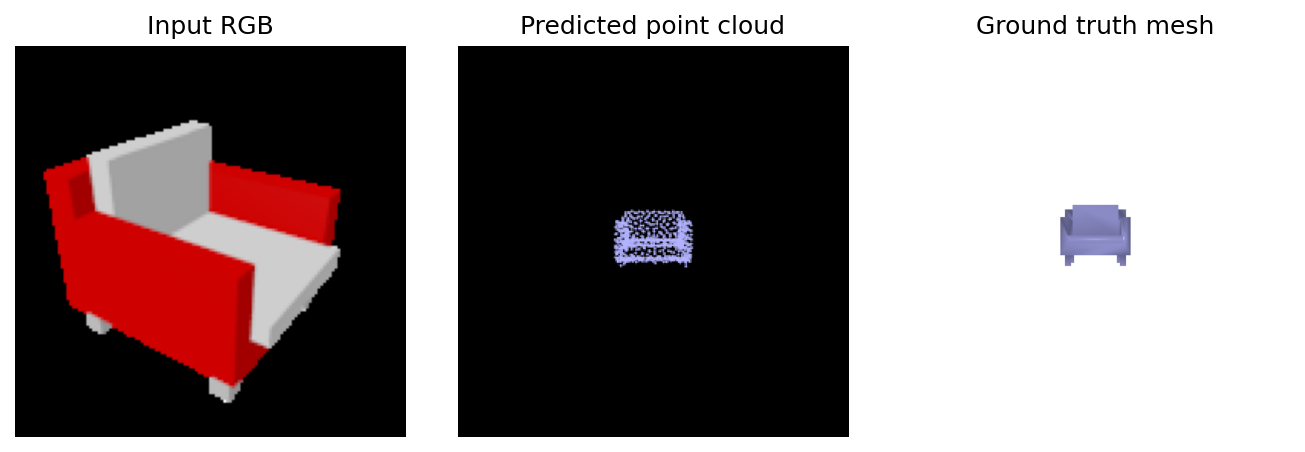
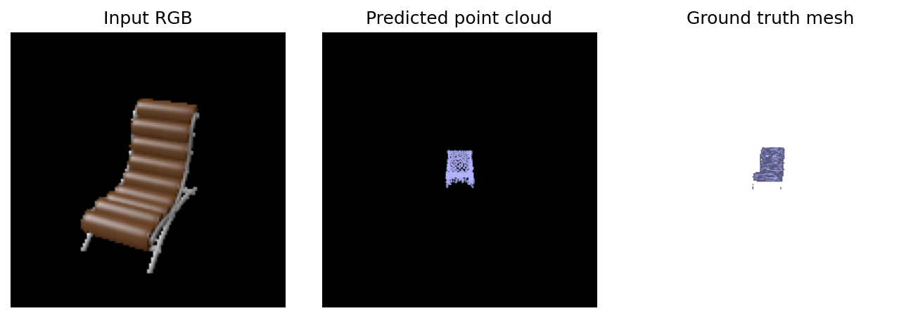
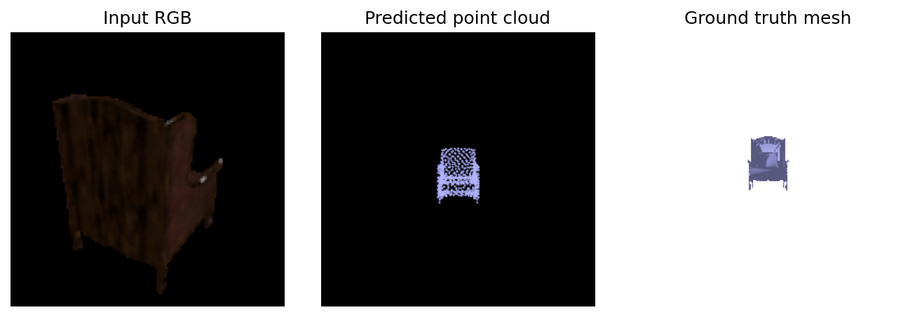
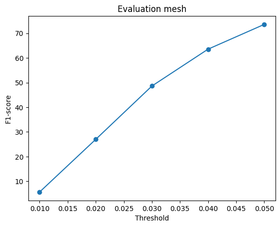
Mesh F1@0.05: 73.58
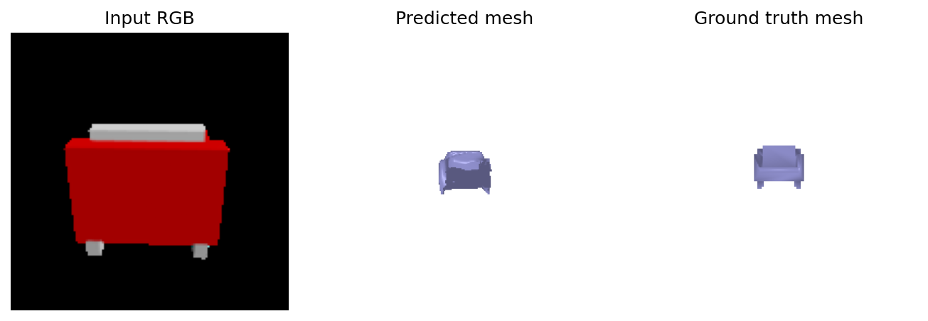
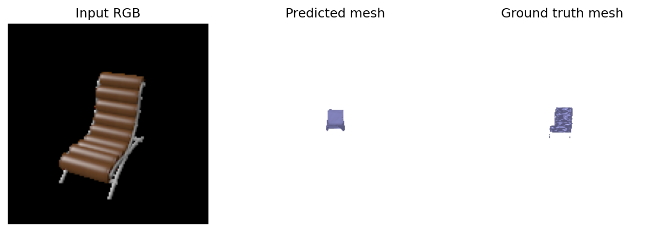
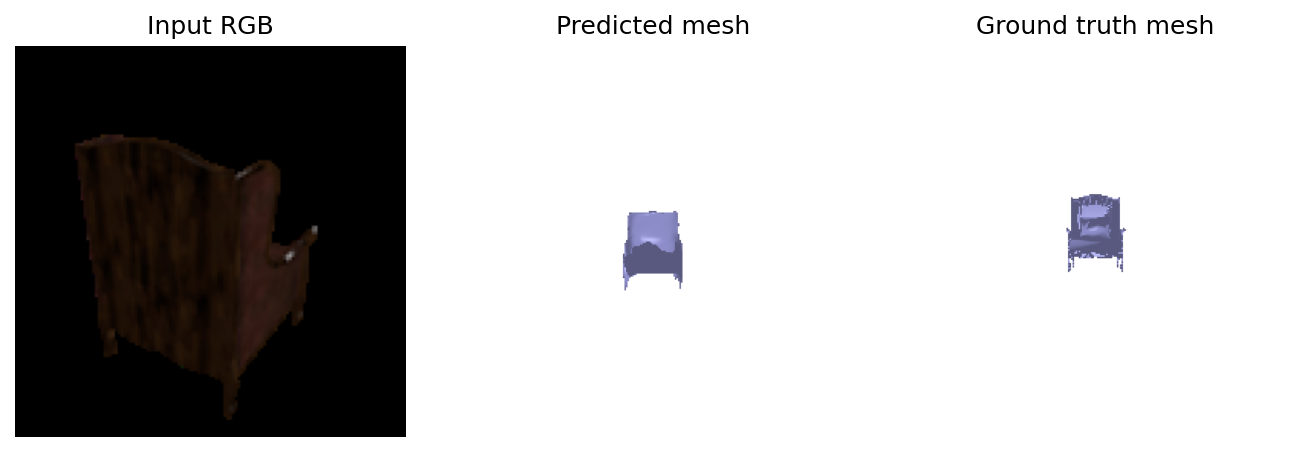
F1@0.05 comparison (Q2): Point cloud (76.20) > Voxel (75.83) > Mesh (73.58). Pointcloud prediction matches the evaluation setup the best. Voxels are limited by the 32³ resolution and marching-cubes error, whereas meshes will struggle with the complex chair surfaces.
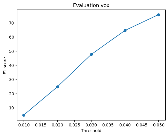
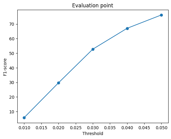
I varied the marching-cubes isovalue on the trained voxel model (the occupancy decision threshold), holding the network fixed. Mean F1@0.05 on the full test set:

F1 rises from 0.2 to 0.65, then drops. A low threshold keeps uncertain voxels, which fattens the surface and hurts precision. Too high of a threshold and it hurts recall since actual parts are being discarded. The best threshold is 0.65, slightly above the default 0.5, suggesting the decoder is tends to assign higher occupancy values than the ground truth. The gain over 0.5 is only about 0.1 F1, so it's not a large free improvement.
Created several slices along different axes of the voxel model and visualized the occupancy grid with respect to ground truth. We see that the prediction has high occupancy in the center of the seat components but has a fuzzy boundary band. In the XY slice the GT has an open gap between seat and back but the prediction tends to fill a bit of it. In general the prediction tends to smooth out the edges and corners and doesn't commit to decisive occupancy values near the boundaries.

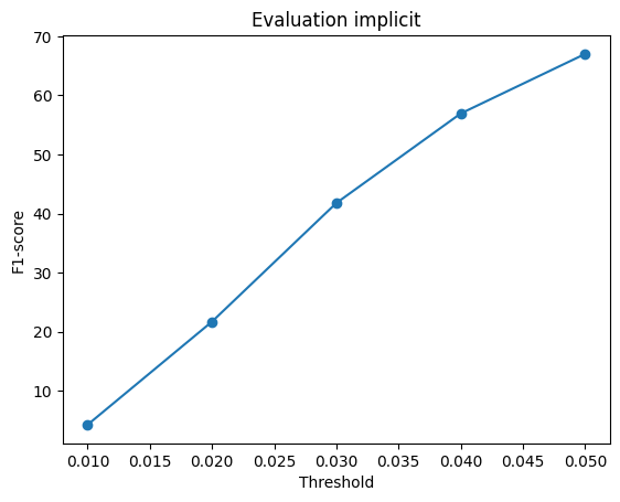
Implicit F1@0.05: 66.99
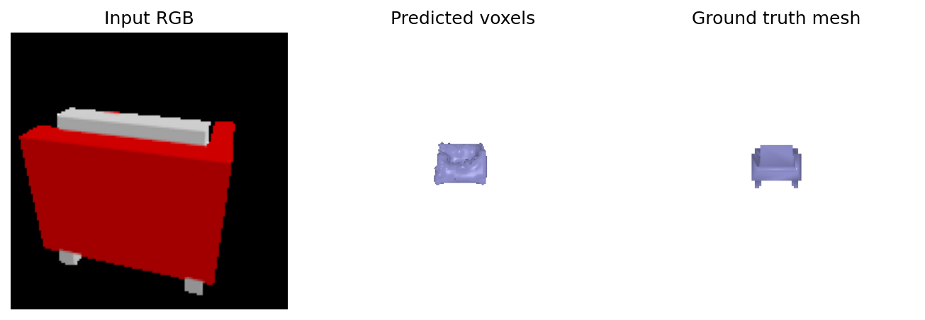
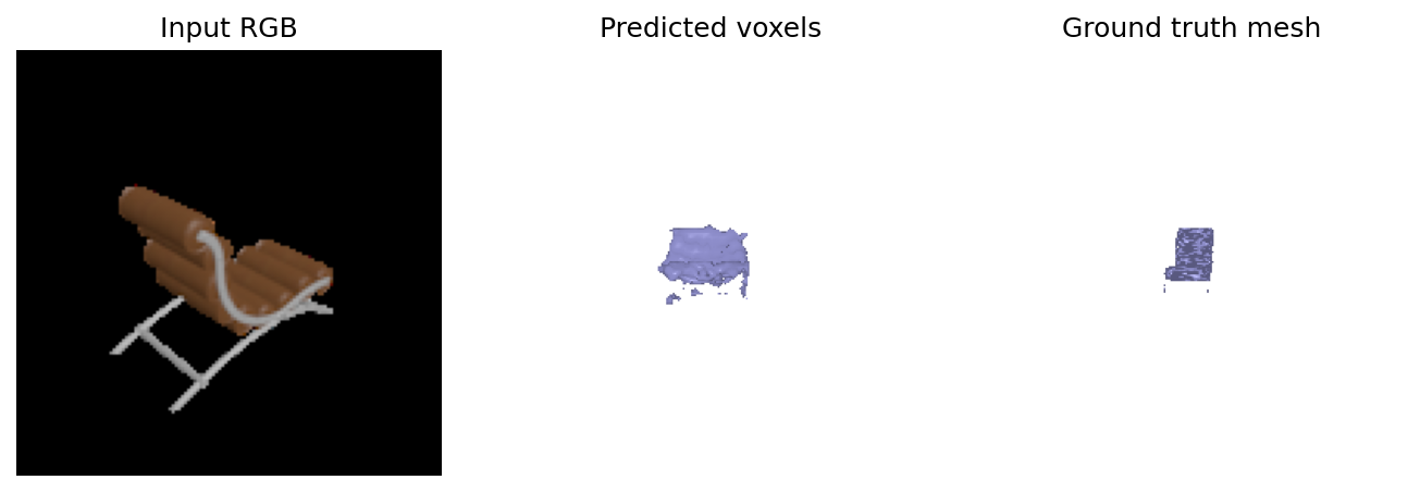
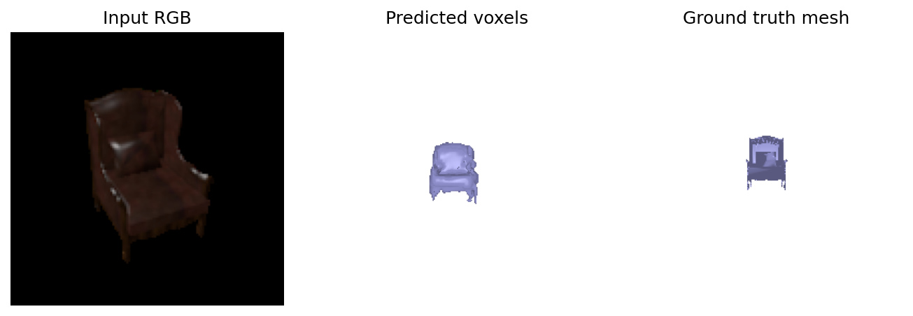
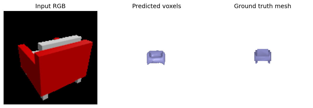
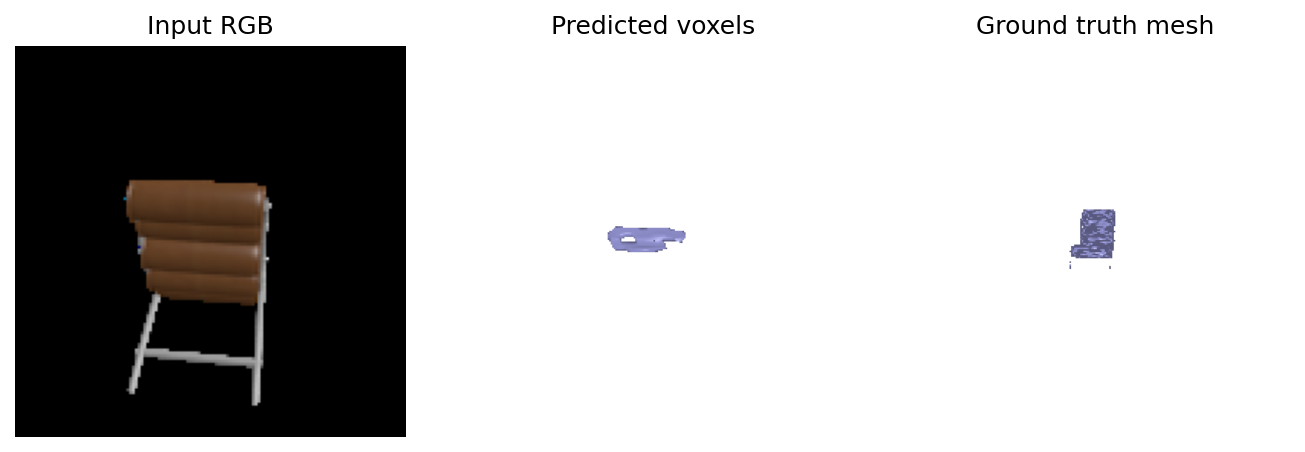
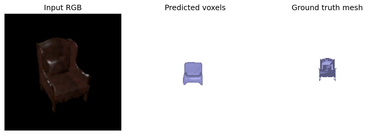
Instead of building the voxel grid with 3D convolutions, this network is a small MLP. For each point on a 32×32×32 grid in (-1, 1), it takes the image feature plus that point's (x, y, z) and predicts whether the point is inside the chair. We then treat those predictions as an occupancy grid like in Q2.1. In terms of performance, the voxel network's conv decoder can use neighboring voxels whereas the MLP sees the same image feature at every point, so it's less stable and a few examples like the second one below fail.
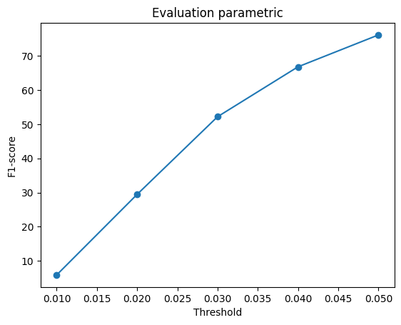
Parametric F1@0.05: 76.09
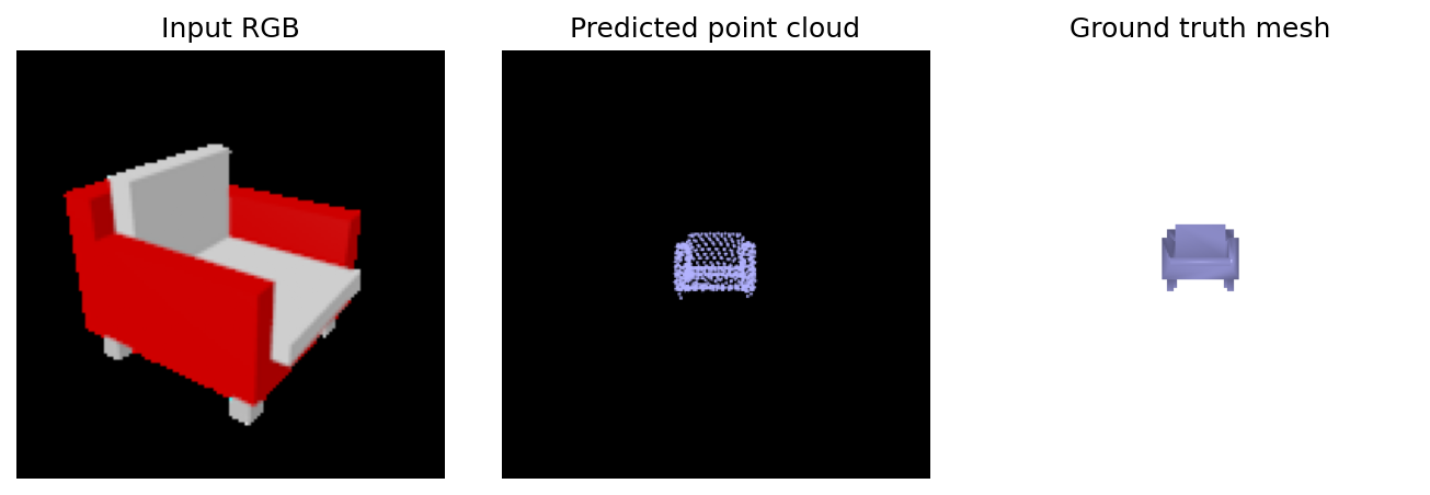
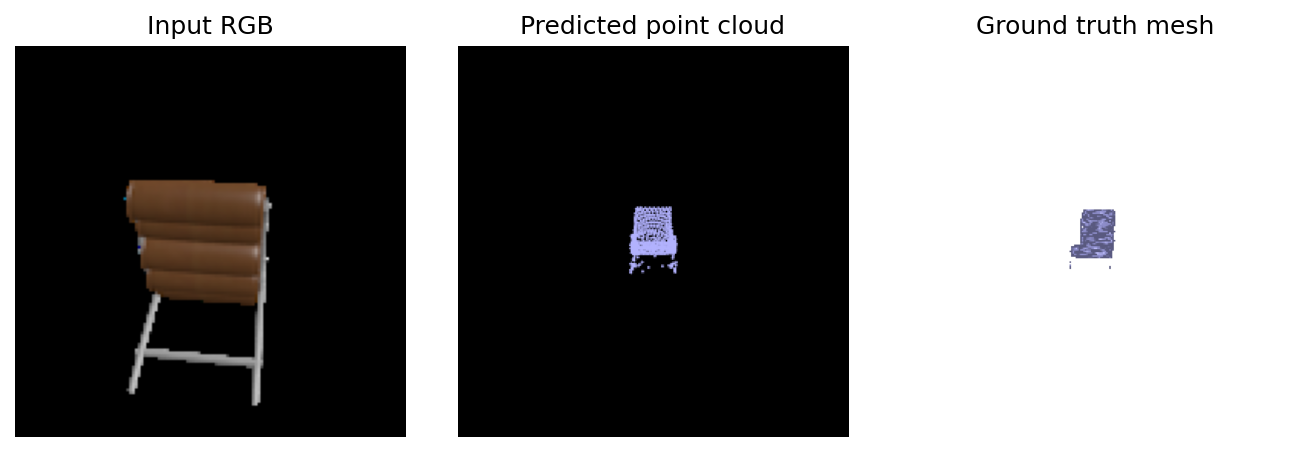
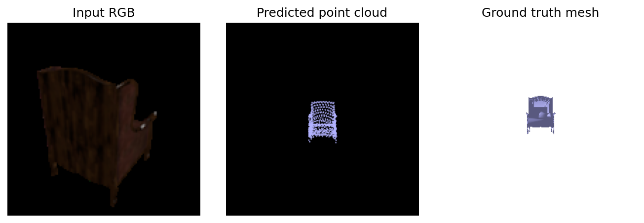
The model predicts a list of 3D points directly from the image by mapping a fixed set of 2D coordinates, split into 4 patches, and a shared MLP maps each 2D coordinate plus the image feature to a 3D point. Nearby 2D samples are supposed to stay nearby in 3D, so the points lie on a surface instead of being an unordered cloud. F1 is almost the same as the point model, but the points are more evenly spaced and the examples look nicer qualitatively.