Assignment 4: Multi-View Transformers
16-825 Learning for 3D Vision
1. Multi-View Data Preprocessing (20 pts)
Implementation. resize_intrinsics scales fx, fy by the size ratio s and maps the principal point with c' = s(c + 0.5) − 0.5, which matches the align_corners=False rule xout + 0.5 = s(xin + 0.5): pixel centres scale about the pixel edges, not about the origin. unproject_depth forms homogeneous pixel centres (u, v, 1), back-projects them with K−1 to the camera-space point at z = 1, multiplies by the z-depth (depth is measured along the optical axis, so no ray-length normalisation is involved), and applies Xw = R Xc + t. canonicalize_cameras left-multiplies every pose by the inverse of camera 0's pose (computed in float64), unprojects depth in that frame, and divides translations, depth and points by the provided scene scale. camera_rays back-projects each pixel with K−1, rotates the result with R (no translation, since it is a direction), normalises it, and uses the camera centre t as the origin. plucker_coordinates returns [d, o × d].
Unprojection (original world frame, metres)


Canonicalisation (first-camera frame, normalised units)
The info panel under each viewer reports the first camera centre (0, 0, 0) and a valid-point centroid distance of 1.000.


check_data.py output (4 training samples)
| Sequence | Views | Res. | Valid depth | Max point reproj. err (px) | Max ray reproj. err (px) | Centroid dist. |
|---|---|---|---|---|---|---|
e050c15a8d_frame_007080 | 8 | 224 | 0.978 | 1.22e-04 | 9.65e-05 | 1.0000 |
5f99900f09_frame_002820 | 8 | 224 | 0.990 | 1.11e-04 | 1.11e-04 | 1.0000 |
47b37eb6f9_frame_002720 | 8 | 224 | 0.961 | 1.26e-04 | 1.11e-04 | 1.0000 |
4c5c60fa76_frame_006690 | 8 | 224 | 0.752 | 1.03e-04 | 9.05e-05 | 1.0000 |
Batch shapes: rgb (2, 8, 3, 224, 224), depth (2, 8, 1, 224, 224), depth_valid (2, 8, 1, 224, 224), K (2, 8, 3, 3), frame_numbers (2, 8), T_world_from_camera (2, 8, 4, 4), original_world_from_reference (2, 4, 4), scene_scale (2,), points_world (2, 8, 3, 224, 224), ray_origins (2, 8, 3, 224, 224), ray_directions (2, 8, 3, 224, 224), plucker (2, 8, 6, 224, 224).
All reprojection errors are around 1e-4 px (the requirement is < 0.01 px), and every sample's centroid sits at distance 1.0.
Explanations
Canonicalisation. Every sample is re-expressed in the coordinate frame of its first sampled camera: T'i = T0−1 Ti, so camera 0 becomes the identity and the arbitrary world frame of each ScanNet++ scan (its origin and orientation) disappears. Then everything with units of length (translations, depth, points) is divided by one shared scale, the distance from camera 0 to the centroid of all valid points, so the scene sits about one unit in front of the reference camera regardless of whether it is a closet or a hall. Rotations, and therefore ray directions, are unchanged by scaling. The centroid is not subtracted: the reference camera stays at the origin. This gives the networks a consistent frame and scale to regress, and removes ambiguities they could not resolve from images anyway (a global rigid transform and the absolute metric scale).
World-space ray directions. For pixel (u, v), K−1(u, v, 1)T is the direction to the point at depth 1 in camera coordinates (OpenCV axes: +X right, +Y down, +Z forward). A world-space direction must ignore the camera translation, so it is rotated by R from Tworld←camera and then normalised to unit length. The origin is the camera centre t. Expressed in the canonical frame, a ray encodes both which pixel it is (intrinsics) and where the camera is relative to camera 0 (extrinsics), so the dense ray map is a per-pixel encoding of the full camera.
Plücker moment. A ray is a line, and Plücker coordinates (d, m) with m = o × d represent the line itself rather than one parametrisation of it. Moving the origin along the ray, o → o + λd, leaves m unchanged because d × d = 0. The direction d says which way the line points; the moment m is perpendicular to the plane containing the line and the world origin, and ‖m‖ is the line's distance to the origin (for unit d). So two rays through the same pixel of cameras at different positions get different moments, while every pixel of a camera at the origin (camera 0) has m = 0. This 6-channel map gives the transformer a smooth, translation-aware camera code it can attend over.
2.1 Mini-LVSM Overfitting (10 pts)
Implementation. patchify reshapes (…, C, H, W) → (L, C, gh, p, gw, p), permutes to (L, gh, gw, p, p, C) and flattens to (…, N, p²C); unpatchify is the exact inverse (I checked the round trip and the row-major patch order). Source tokens are a linear projection of patchified [2·RGB − 1, Plücker] (9 channels); target-query tokens are a separate projection of the target Plücker map only. The fixed 2D sin-cos embedding is added to both. build_tokens flattens the S source views, repeats them for each of the T targets and appends that target's N queries, giving (B·T, (S+1)N, D), so every target is rendered by an independent sequence and targets never see each other. After LayerNorm and 8 transformer blocks, the last N tokens are decoded by LayerNorm → linear → sigmoid → unpatchify. Training runs in bf16 autocast, and predictions are cast to float32 before the MSE loss.

2.2 Training and Evaluation (30 pts)
Settings. Config configs/lvsm.json unchanged: patch size 8, width 384, 8 layers, head dim 64, MLP ratio 4, QK-norm; S = 2 source views and T = 6 targets from 8-view clips sampled within a 32-frame window, 224 px, batch 4 clips; AdamW (lr 2e-4, weight decay 0.05, β = (0.9, 0.95)), 200 warm-up steps then cosine decay, gradient clip 1.0, bf16 autocast; 100 epochs (56 steps each, 5,600 steps) on one RTX PRO 6000. Training took about 66 minutes of wall time (the epoch time varied with NFS load from other jobs on the node). Validation uses the provided prepared clips (first 32 frames, seed 825).

Ablation: number of source views × target-ray conditioning (validation, best.pt)
| Sources | correct rays | shuffled rays | no rays (zeros) | |||
|---|---|---|---|---|---|---|
| PSNR | SSIM | PSNR | SSIM | PSNR | SSIM | |
| S = 1 | 15.21 | 0.5583 | 11.80 | 0.4873 | 12.45 | 0.5266 |
| S = 2 | 16.15 | 0.5603 | 11.48 | 0.4719 | 12.43 | 0.5258 |
| S = 4 | 16.89 | 0.5753 | 11.58 | 0.4724 | 12.44 | 0.5367 |
Training visualisations (columns: source views, ground truth, prediction)


Evaluation visualisations
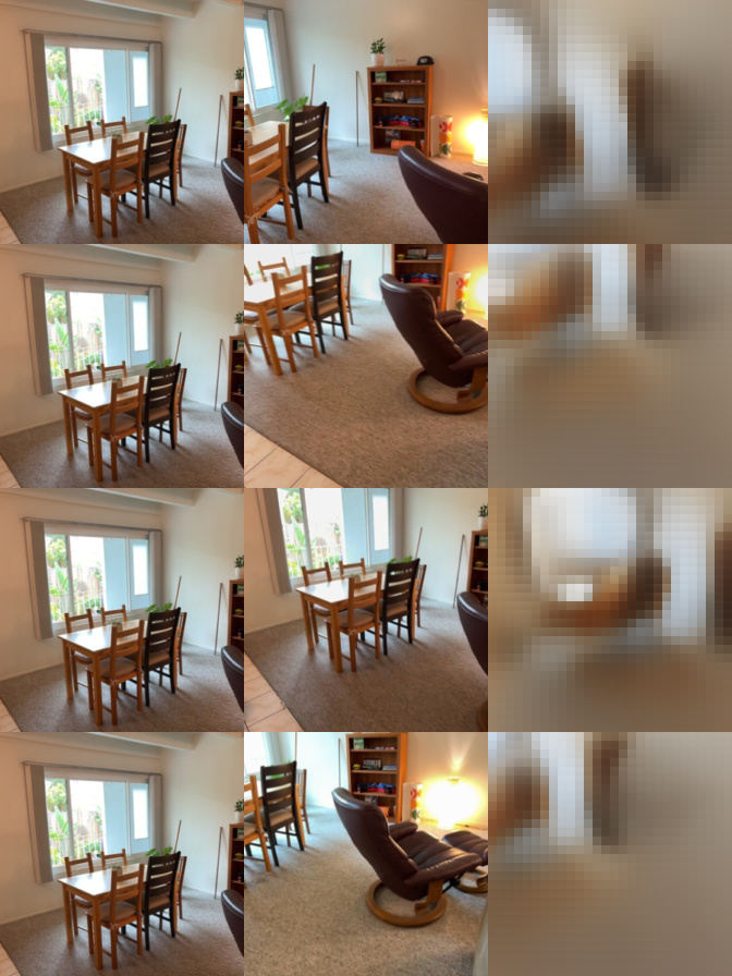

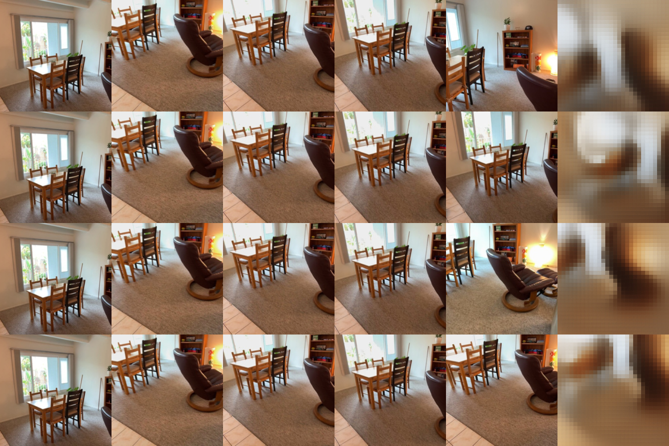
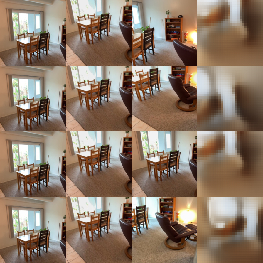

Effect of the number of source views. With the true target rays, quality increases steadily with the number of source views: 15.21 → 16.15 → 16.89 dB PSNR (S = 1, 2, 4), with SSIM following (0.558 → 0.560 → 0.575), even though the model was only ever trained with S = 2. More sources cover more of the target's frustum, so fewer target pixels have to be hallucinated, and multiple observations of the same surface make it easier to triangulate where content belongs. The gain from 1 → 2 sources (+0.9 dB) is larger than from 2 → 4 (+0.7 dB): views from a 32-frame window overlap heavily, so additional sources add progressively less new content. Note the S = 4 evaluation also has fewer targets per clip (4 vs 6), which are closer in time to the sources on average. Visually the predictions are still blurry, with visible 8×8 patch blocks, but they place the window, the dark armchair and the carpet correctly. A 14.6M-parameter model trained for about an hour mainly learns low-frequency, layout-level view synthesis.
Effect of the ray-conditioning ablation. Removing or corrupting the target camera is catastrophic: about 12.4 dB with all-zero rays and about 11.5–11.8 dB with another target's rays, versus 15.2–16.9 dB with the correct rays, at every S. This shows the model really renders from the queried camera rather than memorising a typical frame. With zero rays every query token is identical apart from its positional embedding, so the best the model can do is output a blurry, scene-average colour (the S = 2 panel shows almost uniform beige frames). Ironically that is a safe MSE guess, so it scores slightly better than shuffled rays: with shuffled rays the model confidently renders a sharp-ish prediction of a different viewpoint, and misplaced structure is penalised more than a flat average. Both ablations are flat in S (around 12.4 dB and 11.5 dB), because extra sources cannot help when the network does not know which view to produce. The Plücker conditioning is therefore what carries all the view-specific information.
2.3 Bonus: Training View Count (+10)
Question. Does training with a random number of source views per step (S ~ U{1,2,3,4}, remaining views as targets) generalise better to different source counts at test time than always training with S = 2? Everything else (architecture, data, optimiser, schedule, 100 epochs, seed) is identical, and both models are evaluated with correct rays at S = 1, 2, 4 on the same validation clips.
| Eval sources | trained with S = 2 | trained with S ~ U{1,…,4} | ||
|---|---|---|---|---|
| PSNR | SSIM | PSNR | SSIM | |
| S = 1 | 15.21 | 0.5583 | 15.29 | 0.5595 |
| S = 2 | 16.15 | 0.5603 | 16.25 | 0.5594 |
| S = 4 | 16.89 | 0.5753 | 17.12 | 0.5742 |

Results and discussion. Random-S training gives slightly higher PSNR at every evaluated S: +0.08 dB at S = 1, +0.10 dB at S = 2, and the largest gain, +0.23 dB, at S = 4. SSIM, however, is essentially unchanged (within ±0.001; marginally higher at S = 1 and marginally lower at S = 2 and 4), so the improvement is in per-pixel colour accuracy rather than structure. So training on varied source counts does not trade off the S = 2 case it shares with the baseline, and it helps most where the fixed-S model is out of distribution: the baseline never saw sequences with 4 source views (5N tokens of context), so it has never learned to merge evidence from that many sources, whereas the random-S model saw them 25% of the time. The S = 1 gain is small. A single source is information-limited, so both models are near the same ceiling. Limitations. The differences are small (0.1–0.2 dB) and come from a single seed. The validation curves show both runs still improving at epoch 100, so the ranking could change with longer training. The random-S run also sees fewer target images per step on average (T = 8 − S), which acts as a mild regulariser and is a confound I did not control for. The cost is negligible: the same number of steps, and slightly shorter sequences on average when S < 2.
3.1 Mini-VGGT Overfitting (10 pts)
Implementation. aggregate alternates frame attention (tokens reshaped to (B·V, N, D) with per-view 2D RoPE positions) and global attention ((B, V·N, D) with the same positions repeated per view; no view-order embedding, camera 0 is identified only by its own camera/register tokens). It concatenates the last frame-block output with the last global-block output → LayerNorm → (B, V, N, 2D). The camera head's MLP output keeps translation and quaternion linear and applies ReLU to the two FoV channels (in float32). The depth head maps each patch feature to a p×p depth patch, reassembles the image, adds a zero-initialised RGB-conditioned conv refinement as a residual, and returns depth = exp(·) and confidence = 1 + exp(·). Losses: camera = translation L1 (clamped at 100) + quaternion L1 + 0.5·FoV L1 against the GT encoding; depth = trimmed-mean L1 + trimmed-mean(c·|e| − 0.2 log c) + a 4-scale gradient loss on the masked residual (using torch.where so the graph survives frames with no valid edges).


On the single fixed training clip, the total loss drops from 5.5 to below zero within 40 epochs (the confidence term −0.2·log c becomes negative once the model is confident). Camera loss falls to about 0.003 and pose AUC@30 reaches 0.998 on that clip. The predicted point cloud is visually indistinguishable from the GT: the first camera lands at (−0.0003, 0.0002, −0.0001) instead of the origin, and the centroid distance is 0.997 instead of 1. This confirms that the attention, heads and losses are wired correctly before training on the full split.
3.2 Training and Evaluation (30 pts)
Settings. configs/vggt.json with one change: 300 epochs instead of 1000 (time budget; 10 warm-up epochs, then cosine decay to 5% of the peak lr, with the schedule compressed accordingly). Everything else is default: frozen DINOv2 ViT-B/14, width 384, 6 heads, 8 frame/global pairs, a 4-block camera head, AdamW at lr 6e-4 with weight decay 0.01, batch 16 clips of 8 views from a 32-frame window, 224 px, loss weights camera 5 / depth 1, bf16. Trained on a single RTX PRO 6000 (about 10 s per epoch once data and checkpoints were moved to node-local NVMe), about 55 minutes in total. best.pt is epoch 264 (lowest validation loss).

Metrics (best.pt, 8 views from the first 32 prepared frames, 224 px, seed 825)
| Metric | Validation | Test |
|---|---|---|
| Depth AbsRel ↓ | 0.1639 | 0.1791 |
| Depth δ1 ↑ | 0.7825 | 0.7403 |
| Rotation AUC@5° ↑ | 0.117 | 0.128 |
| Rotation AUC@15° ↑ | 0.355 | 0.381 |
| Rotation AUC@30° ↑ | 0.555 | 0.609 |
| Translation AUC@5° ↑ | 0.016 | 0.006 |
| Translation AUC@15° ↑ | 0.058 | 0.038 |
| Translation AUC@30° ↑ | 0.134 | 0.122 |
| Joint pose AUC@5° ↑ | 0.003 | 0.001 |
| Joint pose AUC@15° ↑ | 0.040 | 0.019 |
| Joint pose AUC@30° ↑ | 0.117 | 0.103 |
GT vs prediction on four validation scenes


Errors on held-out scenes. Depth generalises reasonably to unseen rooms (AbsRel 0.164 val / 0.179 test, δ1 0.78 / 0.74), and the reconstructions recover the coarse layout of each room: walls, floor, large furniture. However, they are visibly smoother than the GT: thin structures such as chair legs, the table edge in scene 2 and the lamp in scene 0 are bloated or missing, and depth discontinuities bleed into the background. That is expected from 14×14-patch tokens decoded by a light per-patch head. Cameras are the weaker part. Rotation is moderately good (median relative error 20° val / 13° test; AUC@30 0.56 / 0.61), but the translation direction is poor (median error about 49°; AUC@30 0.13 / 0.12), which drags the joint pose AUC down to 0.12 / 0.10. In the viewer this appears as predicted cameras clustered too close together and as per-view point clouds that do not register perfectly (doubled walls in scene 3). Two reasons: the frames come from a short 32-frame window, so baselines are small and the translation direction is ill-conditioned (a few centimetres of error is a large angle), and 300 epochs over 224 scenes is little data for learning metric-free relative pose. The training camera loss only fell from 0.23 to 0.21 over the last 60 epochs as the learning rate decayed, so it had not converged much. The full 1000-epoch schedule (or the iterative camera refinement of the official VGGT) would most likely help most here. Validation and test behave similarly, so there is no sign of overfitting to the training scenes; the gap is under-fitting.
3.3 Bonus: Number of Input Views (+10)
Question and setup. How does the number of input views affect Mini-VGGT's accuracy, runtime and memory? The model trained with 8 views (Q3.2 best.pt) is evaluated on the full validation split with 2, 4, 8, 16 and 24 views, all sampled from the same first 32 prepared frames (224 px, seed 825; the reference frame is always view 0). Runtime and memory are measured separately as the latency of a pure forward pass (batch 1, bf16, mean of 10 runs after warm-up) and the peak allocated memory, on real clips for 2–24 views and on synthetic 224 px inputs for up to 256 views.
| Views | AbsRel ↓ | δ1 ↑ | Rot AUC@15 ↑ | Trans AUC@15 ↑ | Pose AUC@15 ↑ | Pose AUC@30 ↑ | ms / sample | Peak GPU mem (GB) |
|---|---|---|---|---|---|---|---|---|
| 2 | 0.1287 | 0.8160 | 0.395 | 0.036 | 0.024 | 0.121 | 22 | 0.74 |
| 4 | 0.1523 | 0.7948 | 0.323 | 0.065 | 0.048 | 0.120 | 21 | 0.76 |
| 8 | 0.1639 | 0.7825 | 0.355 | 0.058 | 0.040 | 0.117 | 21 | 0.81 |
| 16 | 0.2002 | 0.6846 | 0.316 | 0.046 | 0.031 | 0.097 | 21 | 0.89 |
| 24 | 0.1920 | 0.7071 | 0.327 | 0.045 | 0.031 | 0.100 | 22 | 0.97 |
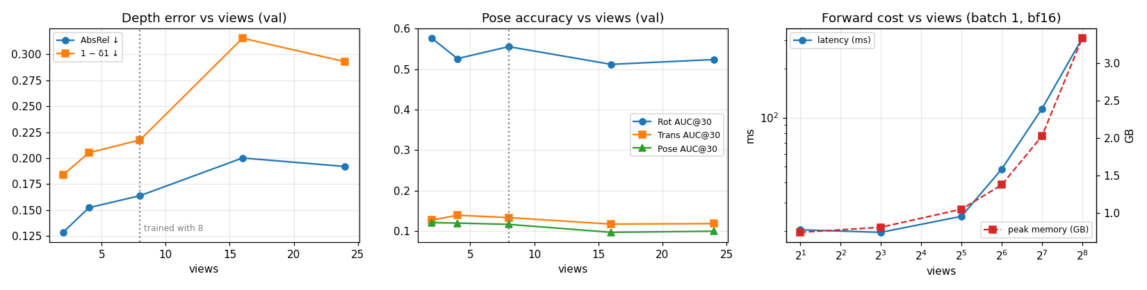
Results and discussion. Depth gets worse as views are added: AbsRel 0.129 (2 views) → 0.164 (8) → 0.200 (16). Part of this is the protocol: the scene scale is the centroid distance of all selected views, so with more views the normalisation covers more of the room and each view's depth has to be predicted relative to geometry it cannot see. Part is the model: global attention was only trained on 8×261-token sequences, and beyond that the attention statistics shift (out-of-distribution sequence length). Pose follows a similar pattern. Rotation and translation AUC@30 are roughly flat from 2 to 8 views and drop at 16–24, while AUC@15 peaks at 4 views (0.048). More views give more pairs to evaluate, including wider-baseline pairs that are harder, so these numbers are not perfectly comparable across rows. Runtime is essentially constant at about 21 ms from 2 to 32 views: at batch 1 the forward pass is launch/overhead-bound (16 attention blocks plus a frozen ViT-B, with the GPU mostly idle). Beyond that, the quadratic cost of global attention over V×261 tokens dominates: 48 ms at 64 views, 113 ms at 128 and 309 ms at 256 (each doubling costs 2.3–2.7×). Memory grows linearly, from 0.74 GB to 3.3 GB at 256 views (about 10 MB per view), because PyTorch's fused SDPA kernel never materialises the attention matrix; the 0.7 GB floor is the weights. Conclusion. The model is cheap enough to run on hundreds of views, but it is accurate only near the view count it was trained on. Training with a random number of views per batch (as in my LVSM bonus) would be the natural fix. Limitations: a single checkpoint and seed, and the 16- and 24-view rows use batch 1 in the metric evaluation. This does not change the metrics, but the views are drawn from the same 32-frame window, so they become more redundant as V grows.