Assignment 3: Neural Volume Rendering & 3D Gaussian Splatting
16-825 Learning for 3D Vision
Everything in Part 4 and Part 7 was implemented: 4.1, 4.2 and 4.3, and both 7.1 and 7.2. All numbers on this page are read from the JSON files written by the training scripts. NeRF/VolSDF PSNRs are averaged over the 100 held-out views of each scene; Gaussian-splatting PSNR/SSIM come from the provided evaluation code.
1. Differentiable Volume Rendering
1.3 Ray sampling (5 pts)
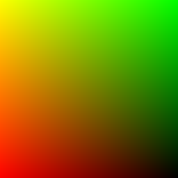
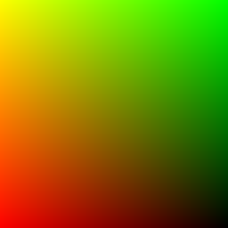
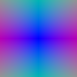
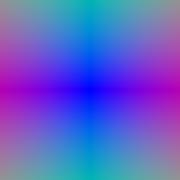
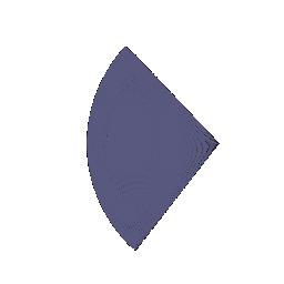
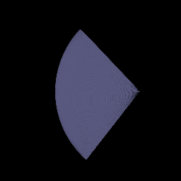
Pixel i of a W-pixel row is mapped to its centre in NDC, x = (2i + 1)/W − 1. PyTorch3D's NDC puts the
image edges at ±1, so pixel centres sit at ±(1 − 1/W). The ground-truth colours are looked up at the same points with
grid_sample(align_corners=False), which returns exact pixel values. The point (xndc, yndc, 1) is
unprojected to world space with camera.unproject_points. The ray origin is the camera centre and the direction is the
normalised vector from the centre to that point. Both visualisations are pixel-identical to the TA's.
1.4 Point sampling (5 pts)
StratifiedRaysampler places n_pts_per_ray evenly spaced depths between
min_depth and max_depth and returns o + t·d for each. While a network is being optimised, each depth is
also jittered uniformly inside its bin (stratified sampling), so the network never sees one fixed set of depths.
Rendering uses the deterministic grid.
1.5 Volume rendering (20 pts)
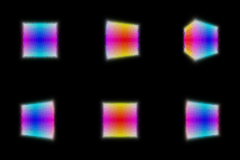
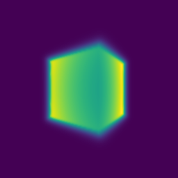
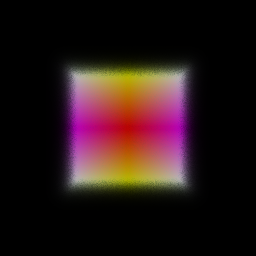
For each segment the opacity is αi = 1 − exp(−σiΔti) and the transmittance is Ti = exp(−Σj<i σjΔtj), computed as an exclusive cumulative sum in log space, so T1 = 1. The weights wi = Tiαi composite both colour (Σ wici) and depth (Σ witi, the expected distance at which the ray terminates). The depth map is normalised by its maximum. The spiral GIF and the depth map are pixel-identical to the TA's.

2. Optimising a Basic Implicit Volume
2.1 Random ray sampling & 2.2 Loss (10 pts)
get_random_pixels_from_image draws a random permutation of all pixel coordinates and keeps the first
n_pixels, so each iteration supervises a different subset of rays with no repeats. The loss is the
mean-squared error between rendered and ground-truth colours (1000 epochs, 4096 rays, Adam at lr 5e-4).
| Pixel convention | Centre (raw) | Side lengths (raw) |
|---|---|---|
| Pixel centres, (2i+1)/W − 1 (used) | 0.2498, 0.2500, -0.0000 | 2.0000, 1.4996, 1.5019 |
| First/last pixel at ±1, 2i/(W−1) − 1 | 0.2502, 0.2504, -0.0003 | 2.0050, 1.5027, 1.5054 |
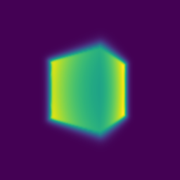
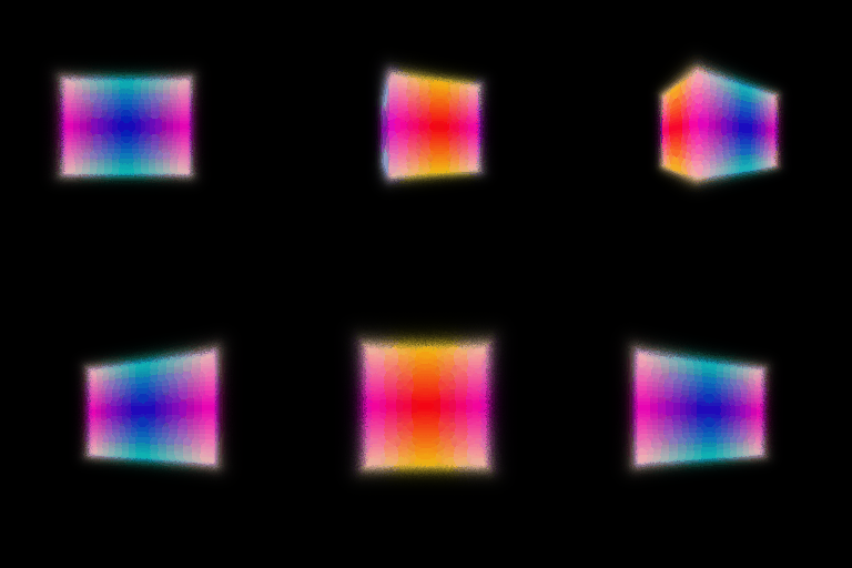
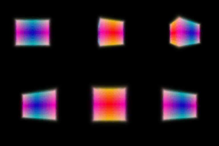
The recovered box depends measurably on the pixel convention. With pixel centres, the box comes out at (0.25, 0.25, 0.00) with sides (2.00, 1.50, 1.50) to within 0.002. With the older mapping, where the first and last pixel sit on ±1, every side comes out about 0.3% too long, and one side rounds to 1.51. That error is the expected one: the older mapping spreads W pixel rays over a field of view that is W/(W−1) = 256/255 ≈ 1.004 times too wide, so the box has to grow by the same factor to cover the same pixels. This is why I use pixel centres everywhere.
2.3 Visualisation

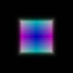
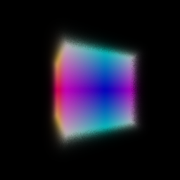


3. Optimising a Neural Radiance Field (20 pts)
Architecture. Positions are encoded with 6 harmonic frequencies (sin/cos plus the raw coordinates, 39-D).
A 6-layer, 128-unit ReLU MLP processes the encoding and re-injects it at layer 3 (skip connection). A linear
head with ReLU gives the density σ ≥ 0. A second branch (linear bottleneck → 64-unit hidden layer
→ 3 outputs with Sigmoid) gives colour. The loss is MSE on 1024 random rays per step. Training uses
Adam (lr 5e-4, decayed ×0.8 every 50 epochs) for 250 epochs at 128×128 with 128 stratified samples per ray between depths 2 and 6.
Getting it to train. My first run rendered an all-black image. On the black-background lego scene the early gradients push every density pre-activation below zero, after which ReLU passes no gradient and the network stays empty. Initialising the density bias to a small positive value (0.1) keeps the ReLU active at the start and fixes this. Nothing else in the setup changed.
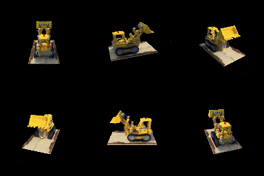
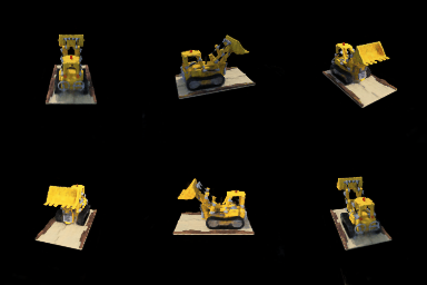

Where does the remaining error come from?
| Lego, 250 epochs | Params | Train PSNR | Held-out PSNR |
|---|---|---|---|
| Q3 model above (128 wide, pixel centres) | 117764 | 24.63 | 24.38 |
| Same model, earlier pixel convention* | 117764 | 24.84 | 24.61 |
| No depth jitter during training* | 117764 | 24.86 | 24.56 |
| 256-wide MLP* | 431876 | 25.76 | 25.37 |
* Diagnostic runs made before switching to pixel centres (Q1.3). The convention itself does not change PSNR measurably (first two rows).
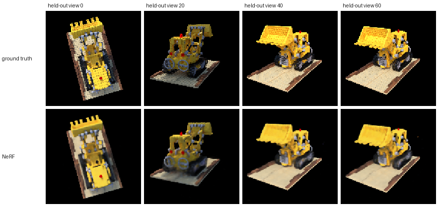
Train and held-out PSNR are within 0.4 dB of each other in every run, so with 100 densely spaced training views the model is underfitting, not overfitting. The remaining error is capacity and resolution, not generalisation. Two checks agree. Removing the depth jitter changes nothing (the jitter protects against aliasing between fixed sample depths, not against overfitting here). Doubling the width to 256 units, with 3.7× the parameters, raises both numbers by about 0.8 dB. I kept the standard 128-unit model so that Q3, Q4.1 and Q4.2 compare like with like. The held-out views show where the error is: fine texture is smoothed away, such as the stud pattern on the bucket and the base plate, the tread links and the small grey pins, while the overall shape and colours are right. Six positional-encoding frequencies in a 128-unit network cannot represent that detail sharply.
4.1 View Dependence (extra credit)
The viewing direction gets its own harmonic embedding (Ldir frequencies) and is concatenated
with the trunk feature only in the colour branch, so density still depends on position alone. This follows
the NeRF design: every view must share the geometry, so only the comparatively low-capacity colour head can
explain view-dependent effects. All models were trained on the materials scene with the provided settings
(nerf_materials.yaml: 128×128, 250 epochs, lr 1e-4).
| Model | Params | Train PSNR | Held-out PSNR | Gap |
|---|---|---|---|---|
| Position only (no view dependence) | 117764 | 23.48 | 23.38 | 0.11 |
| View dependent, Ldir = 2 | 118724 | 24.27 | 24.12 | 0.15 |
| View dependent, Ldir = 6 | 120260 | 24.33 | 24.18 | 0.15 |
View dependent, Ldir = 2, 400×400 (nerf_materials_highres.yaml) | 118724 | 24.40 | 24.28 | 0.12 |
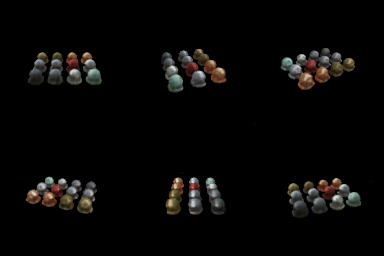
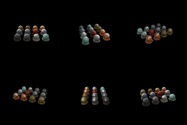
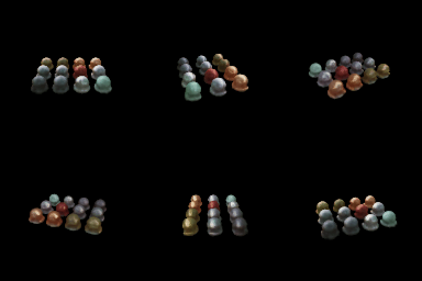


Trade-offs. View dependence raised held-out PSNR on materials by 0.74 dB (23.38 → 24.12 with Ldir = 2). The visual change is where you would expect. The position-only model has to bake a single average colour into each point, so the glossy and metallic spheres look flat and their highlights are smeared into the albedo. The view-dependent models put brighter, tighter highlights on top of the glossy spheres (clearest on the copper and white ones in view 20), and in the GIFs the highlights slide across the surfaces as the camera moves. Away from the highlights, the error maps of the three models look much the same. None of the models reproduces the sharp mirror reflections on the chrome spheres (see the ground truth). A reflected environment is a very high-frequency function of direction, which neither 2 nor 6 frequencies at 128×128 can represent.
The risk of view dependence is generalisation. With enough directional capacity, the colour head could explain each training image separately (the shape–radiance ambiguity), for example by painting view-specific colour onto wrong or semi-transparent geometry. That fits the training images but breaks between them. The train–held-out gap shows the effect, though it is small here: 0.11 dB without view dependence and 0.15 dB with it. Training PSNR rose a little more than held-out PSNR. Two design choices keep it small. Density is computed from position alone, so the geometry must agree across all views, and the direction enters only through a thin (64-unit) layer late in the network. Going from Ldir = 2 to 6 bought just +0.06 dB with the same gap, so on this densely and evenly sampled synthetic scene (100 training views around a full sphere) more directional frequencies neither hurt nor helped much. With sparse or unevenly spread cameras I would keep Ldir low, because a high-frequency directional term can only be trusted near the directions it was trained on. The 400×400 model is the sharpest visually and scores 24.28 dB, but it is evaluated at a different resolution, so its number is not directly comparable.
4.2 Coarse/Fine Sampling (extra credit)
Two separate NeRFs are trained. The coarse network is queried at Nc stratified depths. Its weights
wi define a piecewise-constant PDF along the ray, from which Nf more depths are drawn by inverse-CDF
sampling (random during training, evenly spaced quantiles when rendering). The fine network is evaluated on all
Nc + Nf sorted depths and gives the final colour. Both networks are supervised with MSE, as in the NeRF paper.
To separate the effect of where samples go from how many are used, I compare against single networks with 128 and
256 uniform samples. All runs are on lego with the Q3 settings. Timings come from a separate benchmark
(nerf/bench.py) run on an otherwise idle NVIDIA RTX A5000.
| Lego, 128×128, 250 epochs | Network queries / ray | Params | Held-out PSNR | ms / train step | ms / 128² render |
|---|---|---|---|---|---|
| Uniform, 128 samples (Q3) | 128 | 117764 | 24.38 | 17.7 | 99 |
| Uniform, 256 samples | 256 | 117764 | 24.90 | 33.5 | 235 |
| Coarse 32 + fine (32 + 64) | 32 + 96 | 235528 | 24.76 | 18.8 | 135 |
| Coarse 64 + fine (64 + 128) | 64 + 192 | 235528 | 24.95 | 34.7 | 213 |


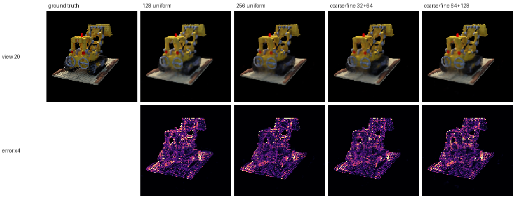
Trade-offs. Quality. At an equal budget of 128 network queries per ray, hierarchical sampling clearly helps. Coarse 32 + fine (32 + 64) reaches 24.76 dB against 24.38 dB for 128 uniform samples. Concentrating samples where the coarse weights are high sharpens the treads, the arm joints and the edges of the bucket (see the error maps). At 256 queries per ray the advantage almost disappears: 64 + 128 gives 24.95 dB against 24.90 dB for 256 uniform samples. On lego at 128×128 the ray segment [2, 6] is short and the object fills much of it, so dense uniform sampling already resolves the surfaces. Importance sampling pays off most when samples are scarce or the scene has a lot of empty space.
Speed. Cost is set mostly by the number of network queries. The 128-query models train at 17.7 vs 18.8 ms per step and the 256-query models at 33.5 vs 34.7 ms, so the extra cost of coarse/fine is a small overhead (about 6%) for building the PDF, inverting it and sorting. Rendering a full image costs more with coarse/fine at the small budget (135 vs 99 ms), because the coarse and fine passes run one after the other. Coarse/fine also doubles the parameters (two networks) and both must be trained. A failure mode remains: if the coarse network misses a thin structure entirely, the fine pass never samples it. Trade-off: for a fixed compute budget, coarse/fine gives better images when samples are scarce. With a generous budget, plain uniform sampling is simpler and about as good.
4.3 VolSDF (extra credit)
Implementation. The distance network is a 6-layer, 128-unit MLP on the 6-frequency positional encoding,
with Softplus (β = 100) activations instead of ReLU so that the SDF and its gradient are smooth. It uses the geometric
initialisation of SAL/IGR: high-frequency encoding inputs are zeroed and the last layer is set so that the
network starts close to the SDF of a unit sphere, d(x) ≈ ‖x‖ − 1. A colour head (2 × 128 ReLU → Sigmoid) takes the
distance network's last hidden feature together with the encoded position, and get_distance_color shares one
trunk pass between the two outputs. The eikonal loss is mean((‖∇d‖ − 1)²) on random points in the [-4, 4]³ box
(weight 0.02). Density is σ(x) = α Ψβ(−d(x)), where Ψβ is the CDF of a zero-mean Laplace distribution
with scale β. Both branches are written in terms of exp(−|d|/β), so the unused branch of torch.where can never
overflow and produce NaN gradients.
Intuition for α and β. α is the density deep inside the object: Ψβ → 1 inside, so α sets how opaque the solid is, and therefore how quickly a ray saturates after it crosses the surface. β is the width of the transition: density falls from α to α/2 exactly at the zero level set and decays to 0 outside over a distance of a few β. As β → 0 the density becomes an indicator function of the interior and the surface becomes a sharp step.
- 1. How does high β bias the learned SDF? What about low β?
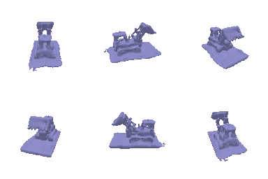
- High β spreads density over a thick band around the zero level set, so each pixel is explained by a fuzzy, semi-transparent shell rather than a surface. Outside the surface the density is already σ = ½α·e−d/β, so rays start absorbing before they reach d = 0, and the optimiser compensates with an SDF whose zero level set is smoothed and pulled away from the true surface. Anything thinner than a few β gets blurred into its surroundings. At β = 0.2 my mesh is visibly over-rounded: the base plate becomes a thick pillow and the cab and tracks lose their edges. The colour is also the blurriest (21.5 dB, versus about 22.4 dB for smaller β at the same α). Low β removes this bias. The density approaches α times an indicator function of the interior, so the rendered surface coincides with the zero level set. The price is that only points very close to the surface get a useful gradient.
- 2. Is an SDF easier to train with volume rendering and low or high β?
- High β is easier to train. The density varies smoothly over a wide band, so many samples along each ray, not just those within a hair of the surface, give gradient to the SDF. The loss landscape is smoother, and coarse ray sampling still lands inside the transition region. With low β the transition can become narrower than the spacing between samples (4 units / 128 samples ≈ 0.03 here, i.e. 3β at β = 0.01). Rays can then step over the surface, the gradients become very peaky, and training leans heavily on a good initialisation. In my runs low β still trained, thanks to the sphere initialisation, the eikonal term keeping |∇d| ≈ 1 and the per-step jitter of the samples. But at α = 10 the low-β runs show the typical failure: small floating fragments and holes in the base plate.
- 3. Is an accurate surface more likely with high or low β?
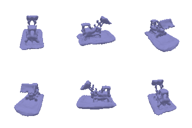
- Low β, provided training converges. When the density is close to a step at d = 0, volume rendering effectively becomes surface rendering, so the image can only be matched by putting the zero level set on the true surface. There is no semi-transparent fuzz left in which to hide errors. One caveat from the sweep: low β pays off only together with a large enough α. With α fixed at 10, an interior density of 10 needs about 0.3 units of travel to become opaque, so thin parts such as the bucket and the base plate cannot become solid however small β is. PSNR is then nearly flat for β ≤ 0.05. Scaling α = 1/β, as the VolSDF paper does, makes the object opaque within a few β of the surface, and β = 0.01 with α = 100 gives by far the sharpest geometry and the best PSNR.
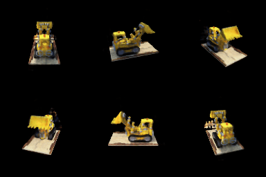
Best result (α = 100, β = 0.01, eikonal weight 0.02, 250 epochs)


Hyper-parameter sweep
| α | β | Train PSNR | Held-out PSNR | |
|---|---|---|---|---|
| 10 | 0.01 | 22.46 | 22.29 | |
| 10 | 0.02 | 22.53 | 22.37 | |
| 10 | 0.05 | 22.61 | 22.44 | default config |
| 10 | 0.2 | 21.62 | 21.46 | |
| 100 | 0.01 | 24.59 | 24.38 | α = 1/β |
| 50 | 0.02 | 24.49 | 24.28 | α = 1/β |
| 20 | 0.05 | 23.46 | 23.27 | α = 1/β |
| 5 | 0.2 | 20.62 | 20.46 | α = 1/β |
β sweep at the default α = 10


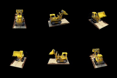

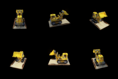
α = 1/β (as in the VolSDF paper)


Chosen settings. The best setting is α = 100, β = 0.01 (24.38 dB held out), with the eikonal weight 0.02 and the schedule of volsdf_surface.yaml. Two things mattered most. (1) The geometric (sphere) initialisation with Softplus activations. It gives a valid SDF from the first step, so the eikonal term is satisfied immediately and rendering starts from a sensible closed surface. (2) Choosing α together with β. With the default α = 10, PSNR is nearly flat for β ≤ 0.05 (22.3–22.4 dB), because an interior density of 10 makes thin parts semi-transparent whatever β is, and the low-β runs grow small floaters. Scaling α = 1/β, as in the VolSDF paper, makes the solid opaque within a few β of the zero level set, and PSNR rises steadily as β shrinks: 20.46 → 23.27 → 24.28 → 24.38 dB for β = 0.2 → 0.01. The geometry shows the same thing: a thin, flat base plate and a clearly separated bucket, arm and treads. The α = 1/β rule is not magic, though. At β = 0.2 it lowers α to 5 and is worse than α = 10 (20.46 vs 21.46 dB). What matters is that the density inside is high enough for the surface to be opaque. I did not go below β = 0.01, because the transition would become narrower than the 0.03-unit sample spacing. Smaller β would need more samples per ray or a coarse-to-fine sampler.
5. 3D Gaussian Rasterisation (35 pts)
Projection (5.1). The 3D covariance is Σ = R S Sᵀ Rᵀ, which for isotropic Gaussians is simply s²I, so
the quaternions are skipped. The 2D covariance is Σ' = J W Σ Wᵀ Jᵀ, where J is the provided perspective Jacobian and W
is the world→camera rotation. PyTorch3D uses row vectors (xview = xworldR + T), so in
column-vector form W = Rᵀ. Means are projected with transform_points_screen.
Evaluation (5.2). The exponent is written out as −½(a·dx² + 2b·dx·dy + c·dy²) from the entries of Σ'−1,
which made rendering about 5× faster than an einsum that lowered to many tiny matrix multiplies.
Filtering, sorting, compositing (5.3–5.5). Gaussians are sorted by view-space depth and those behind the camera (z < 0) are dropped. Per pixel, αi = oiexp(Pi) and Ti = Πj<i(1 − αj), computed with a cumulative product. Colour is Σ ciαiTi, depth is Σ ziαiTi and the silhouette is Σ αiTi (the accumulated opacity). Splatting runs in mini-batches whose transmittance is chained from one batch to the next.
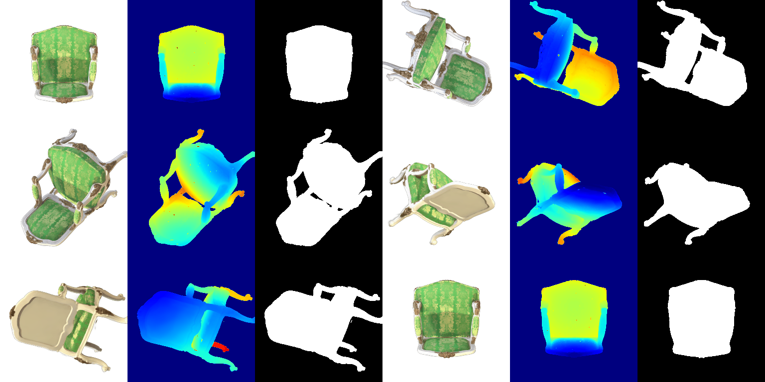
Unit tests and the choice of W
unit_test_gaussians.py passes tests 1 and 3 and fails tests 2 and 4.
With W = R, which is the only line that differs, it passes 4/4. Tests 2 and 4 are the anisotropic-covariance tests, and their
expected values were generated with W = R. The course's reference frame for Q5 (frame 29) also matches a W = R
render to 57.7 dB, and a W = Rᵀ render to
29.8 dB.To check which convention is geometrically right, GS/analysis_w_convention.py samples 200,000 points from each of
8 random, strongly anisotropic 3D Gaussians and projects them with PyTorch3D's own transform_points_screen.
It then compares their empirical 2D covariance with compute_cov_2D. Averaged over three viewpoints, the relative
error is 1.2% with W = Rᵀ and
251% with W = R. The renders agree. At the
reference frame the two conventions look almost the same, because that viewpoint's rotation is close to symmetric. At other frames W = R
smears elongated Gaussians into streaks.


6. Training 3D Gaussian Representations (15 pts)
All Gaussian attributes (means, log-scales, colours, pre-sigmoid opacities) get requires_grad=True. The
Gaussians are isotropic, so the quaternions are not optimised. Each step renders one training view and minimises the L1 loss to the
ground-truth image. Every parameter group has its own Adam learning rate.
Iterations: 5000 · Mean PSNR: 31.56 · Mean SSIM: 0.954
| Run | Means | Scales | Colours | Opacities | Iterations | PSNR | SSIM |
|---|---|---|---|---|---|---|---|
| chosen lrs | 0.0003 | 0.005 | 0.01 | 0.05 | 1500 | 30.20 | 0.945 |
| chosen lrs | 0.0003 | 0.005 | 0.01 | 0.05 | 3000 | 30.79 | 0.950 |
| chosen lrs (final) | 0.0003 | 0.005 | 0.01 | 0.05 | 5000 | 31.56 | 0.954 |
| higher lrs | 0.001 | 0.01 | 0.02 | 0.05 | 1500 | 29.96 | 0.945 |
With the same learning rates, longer training kept improving the held-out views: 1500 → 3000 → 5000 iterations gave 30.20 → 30.79 → 31.56 dB. I report the 5000-iteration run. Raising the means, scales and colour rates (last row) lowered the training loss slightly faster at first but generalised worse (29.96 vs 30.20 dB at 1500 iterations). Larger position steps make the means jitter around their optimum, which shows up as small misalignments on unseen views. The truck's starting point cloud is already accurate, so the means need only small corrections, and a low means rate (3e-4) works best. Opacity and colour start far from their targets (random colours, nearly opaque) and benefit from large steps.
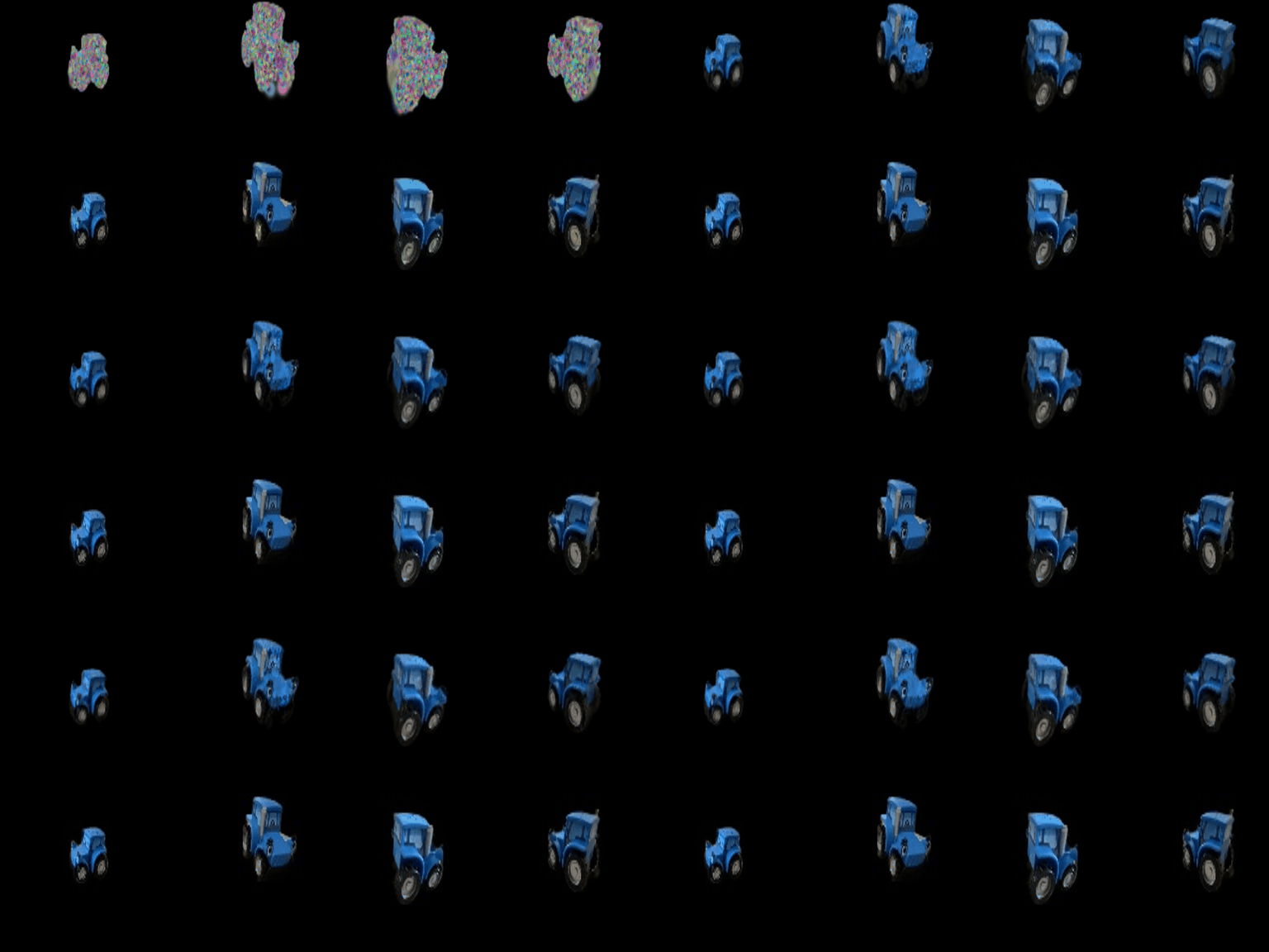

To fit next to other jobs on a shared GPU, training renders in mini-batches of 2500 Gaussians wrapped in
gradient checkpointing (torch.utils.checkpoint). Each mini-batch's per-pixel intermediates are freed after the
forward pass and recomputed in the backward pass. This halves peak memory (about 8 GB to about 4 GB) without changing the output.
7.1 Rendering Using Spherical Harmonics (10 pts)
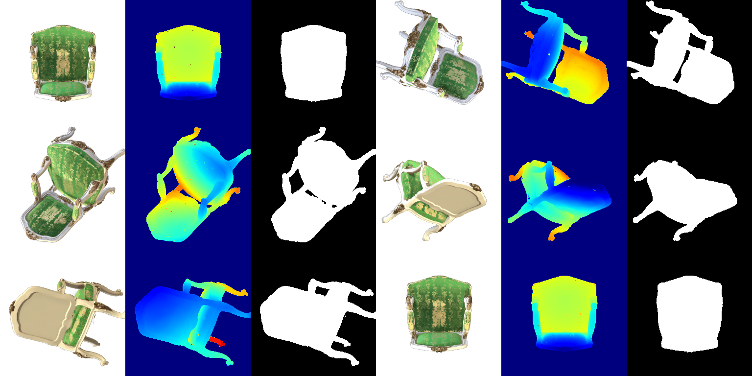
The 48 coefficients per Gaussian are reshaped into 16 RGB coefficients (degrees 0–3) and evaluated with the real SH basis
in the direction from the camera centre to each Gaussian mean, vectorised over all Gaussians. As with the
DC-only colours, 0.5 is added and the result is clamped at 0. render.py --use_sh switches between the two colour models.
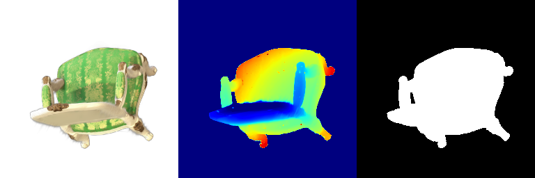
Side-by-side comparisons
Each panel shows: DC only | full SH | per-pixel |SH − DC| × 4 | zoom on the 64×64 window with the largest change (red box). The mean absolute change on the object is 0.097 (frame 0), 0.059 (frame 8) and 0.021 (frame 24), the largest, a middle and the smallest of the 32 frames.
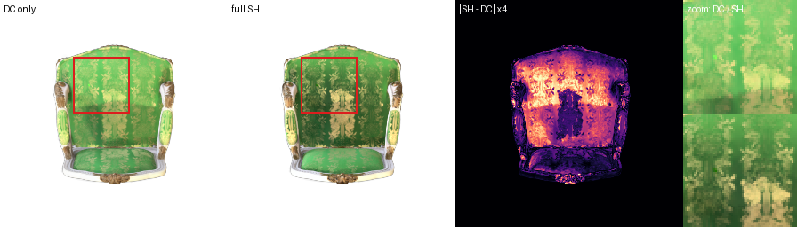
Frame 0. Front view of the backrest. This frame changes the most. With full SH the green brocade is darker and more saturated, and the light damask pattern stands out against it, as sheen fabric does when the light is not reflected straight back at the viewer. The DC-only render shows the same fabric as a flatter, lighter green, because the DC term is roughly the colour averaged over all viewing directions. The difference map is bright over almost the whole upholstered panel and the gilded arm ornaments. It is dark on the white frame and the carved feet.
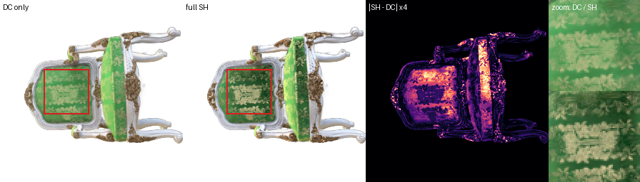
Frame 8. View from above onto the seat and the top of the backrest. The seat fabric again darkens and gains contrast with SH (zoom). The white frame around the seat picks up a thin band of grey shading along its inner edge. In the DC-only image the frame is a uniform flat white, so with SH it reads as more three-dimensional. The gilded corner carvings change too, gaining small view-dependent glints, as a metallic finish should.
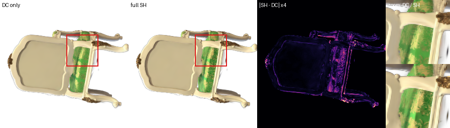
Frame 24. View of the back of the chair. This frame changes the least. The large back panel is matte painted wood, close to Lambertian, so its higher-order SH coefficients are near zero and the DC colour already explains it. The difference map is almost black there. What changes is confined to the strip of green fabric visible at the side and to silhouette edges. Together the three frames show that SH only changes appearance where the material is actually view dependent: strongly on the fabric and gilding, hardly at all on paint.
7.2 Training on a Harder Scene (extra credit)
The materials scene is trained from 10,000 randomly initialised Gaussians. The baseline is exactly the Q6 recipe:
isotropic Gaussians, the Q6 learning rates, L1 loss, init_type="random" and 1500 iterations.
| Method | Iterations | Final # Gaussians | PSNR | SSIM |
|---|---|---|---|---|
| Baseline (Q6 recipe) | 1500 | 10000 | 18.57 | 0.683 |
| Improved (all modifications below) | 5000 | 17777 | 24.76 | 0.903 |
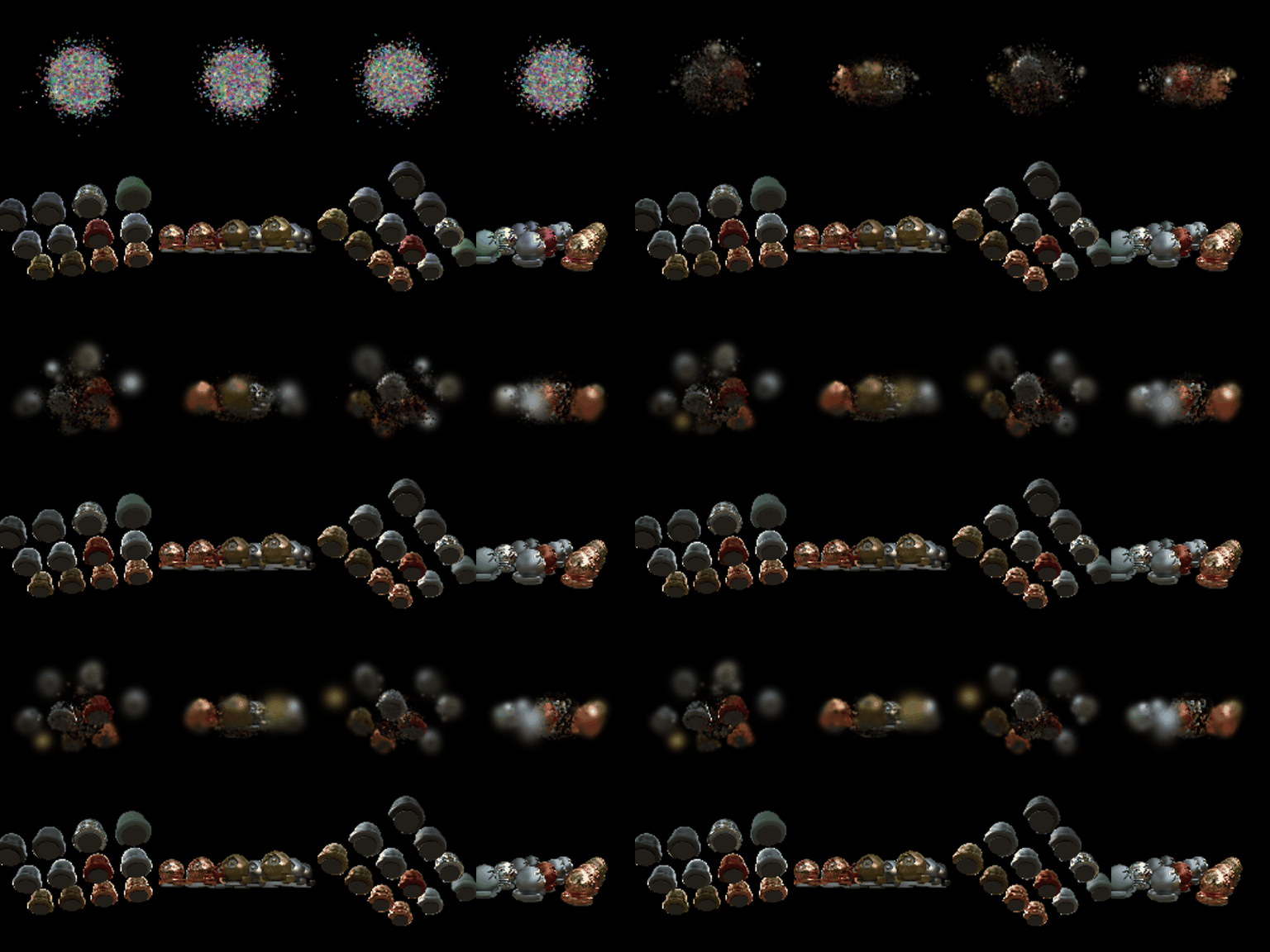
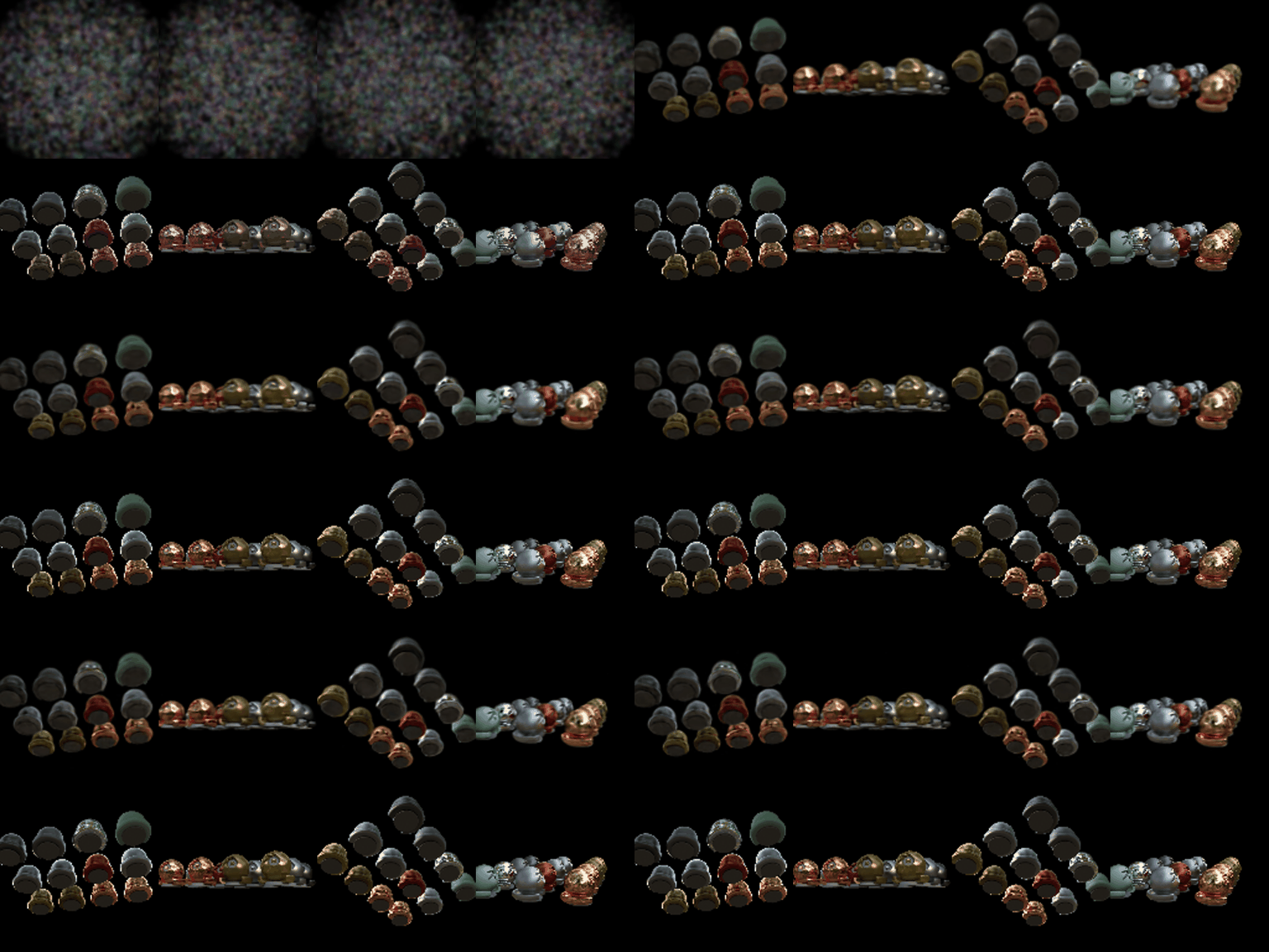

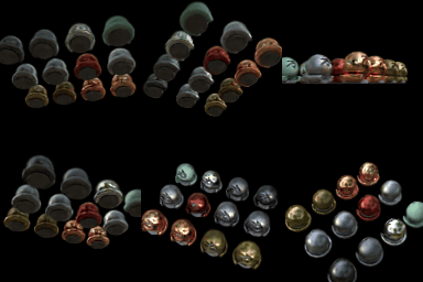
Modifications compared with the Q6 recipe
- Initialisation that covers the scene. The default random init draws means from N(0, 0.2²), a tight ball around the origin, but the materials objects span roughly [-1.5, 1.5]. I sample means uniformly in a ball of radius 1.5 and start every Gaussian at scale 0.03 and opacity 0.1, instead of tiny and nearly opaque. Every pixel then gets gradient from several overlapping, semi-transparent Gaussians, and none of them hides the others early on.
- Position learning-rate schedule. Means start at lr 0.002, about 7× the Q6 value, so they can travel from the random init to the objects. The rate decays exponentially to 1% of that by the end, so late training only refines.
- Anisotropic Gaussians with optimised quaternions (lr 0.001), so that flat surfaces and object silhouettes can be covered by elongated Gaussians.
- L1 + D-SSIM loss, 0.8·L1 + 0.2·(1 − SSIM) with an 11×11 Gaussian window, as in the 3DGS paper.
- Simplified adaptive density control, every 150 iterations from iteration 300 until 60% of training. Gaussians whose mean positional-gradient norm exceeds 0.00035 are cloned if small (max scale ≤ 0.05) or, if large, split into two samples drawn from themselves with their scale divided by 1.6. Gaussians with opacity < 0.005 are pruned, and the total is capped at 30000.
Ablation: what each modification contributes
Each row adds one modification to the row above. All rows are trained for 2000 iterations so that they are comparable. The last two rows remove the initialisation from the full recipe and train the full recipe for longer.
| Configuration | Iterations | # Gaussians | PSNR | SSIM | ΔPSNR vs. row above |
|---|---|---|---|---|---|
| Baseline (Q6 recipe) | 2000 | 10000 | 18.79 | 0.694 | |
| + scene-covering initialisation | 2000 | 10000 | 22.75 | 0.830 | +3.96 |
| + large, decaying means lr | 2000 | 10000 | 22.89 | 0.839 | +0.15 |
| + anisotropic Gaussians | 2000 | 10000 | 23.52 | 0.860 | +0.62 |
| + L1 + D-SSIM loss | 2000 | 10000 | 23.54 | 0.869 | +0.03 |
| + densification = full recipe | 2000 | 11358 | 23.96 | 0.883 | +0.42 |
| full recipe without the new initialisation | 2000 | 15609 | 18.96 | 0.752 | -5.00 |
| full recipe, longer training | 5000 | 17777 | 24.76 | 0.903 | +0.80 |
Result. The final recipe raises PSNR from 18.57 to 24.76 dB (+6.2 dB) and SSIM from 0.683 to 0.903. At 2000 iterations the same recipe reaches 23.96 / 0.883. Training it for 5000 iterations adds another 0.8 dB, and densification grows the scene to 17.8k Gaussians. The ablation shows that the initialisation is the change that matters. On its own it adds about 4 dB (18.79 → 22.75), and the full recipe without it scores only 18.96 dB, barely above the baseline. The baseline never escapes its initialisation. All 10k Gaussians start in a tight ball (σ = 0.2) at the centre while the objects fill a much larger area, and with the small Q6 means rate the Gaussians can travel only about 0.0003 per step. The middle objects form, but the outer ones stay as blurry, glowing blobs, as the baseline's training-progress GIF shows. The other modifications only help once the Gaussians are near the objects. Anisotropic Gaussians add the most after that (+0.63 dB), because elongated Gaussians can follow the spheres' silhouettes and the thin pedestals. Densification adds +0.42 dB and 0.014 SSIM by cloning or splitting Gaussians that still have large positional gradients (mostly on object edges) and pruning near-transparent floaters left over from the uniform initialisation. The decaying means rate (+0.14 dB) and the D-SSIM term (+0.02 dB, but +0.009 SSIM, the quantity it targets) are small refinements. With the improved recipe the first few hundred iterations already produce a recognisable layout. Limitations. The remaining errors are on the metallic and glossy spheres, whose reflections and highlights a view-independent colour cannot represent (training SH coefficients would be the natural next step), and on thin rims.