Single View to 3D
Fitting a voxel grid
We optimize a 32³ grid of occupancy logits using binary cross-entropy. After 2,000 Adam updates, the thresholded prediction matches every target voxel (IoU = 1.000).
The binvox axes are mapped as (x, y, z) → (z, y, −x) before aligning the occupied cell bounds to the mesh. We sample each target cell by inverse mapping. The voxel grid is coarser than the original mesh, but has no artificial slit.

Fitting a point cloud
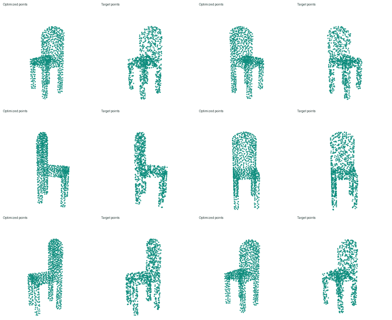
We initialize 1,000 points from a Gaussian with standard deviation 0.25 and optimize them for 5,000 updates. The target contains 10,000 points sampled uniformly over the mesh surface.
LChamfer = meanp ∈ P minq ∈ Q ‖p − q‖² + meanq ∈ Q minp ∈ P ‖q − p‖²
We compute the nearest neighbors with knn_points and implement both reductions in losses.py.
Fitting a mesh
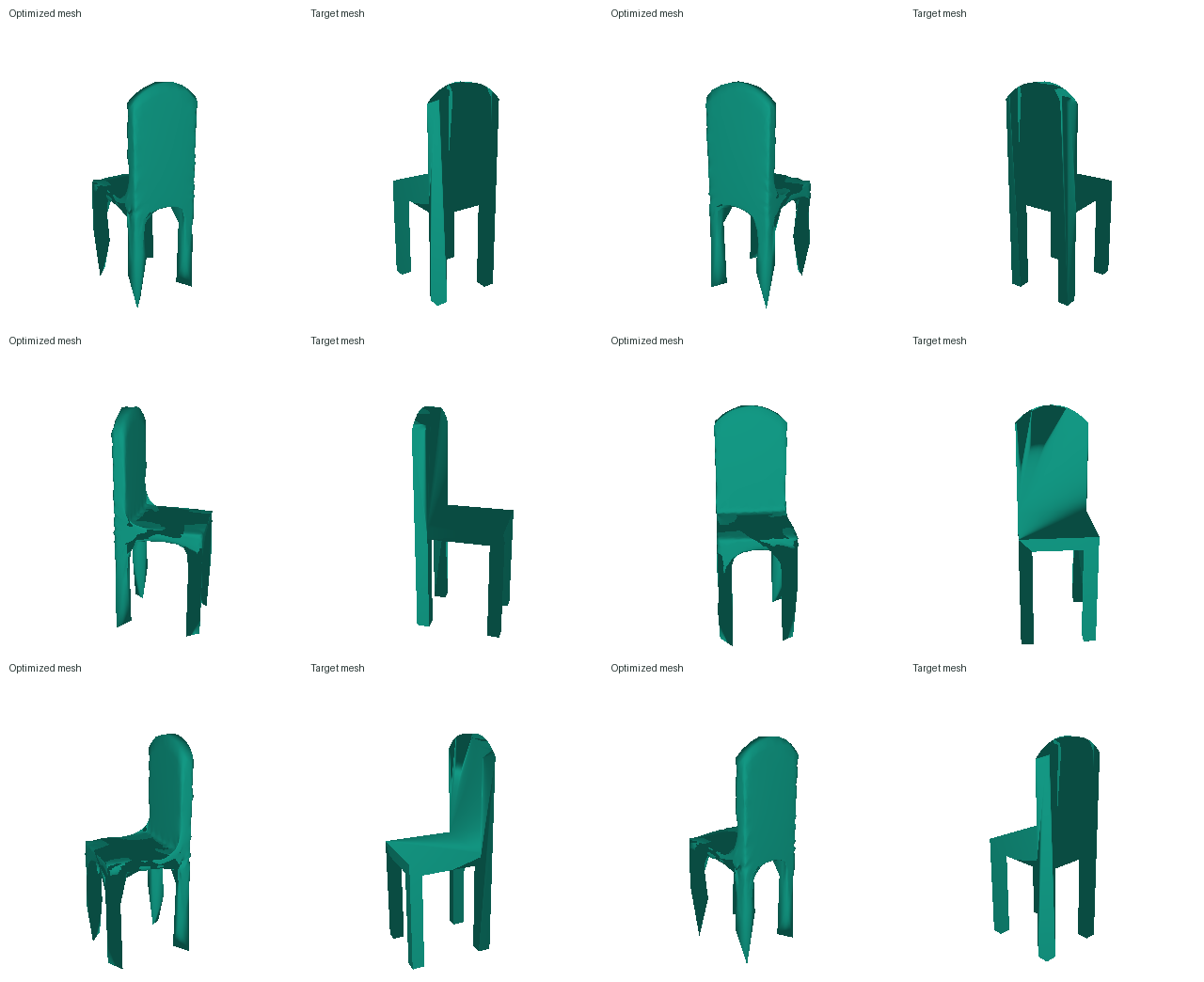
We start from a level-4 icosphere with 2,562 vertices and optimize vertex offsets for 7,000 updates. The loss is Chamfer distance plus 0.1 times the uniform Laplacian loss. The Laplacian term penalizes the distance between each vertex and the mean of its neighbors.
Reconstructing 3D from a single view
The dataset contains image–shape pairs. Each chair has a mesh, a 32³ voxel grid, and ten rendered RGB views. Every complete training pass includes all ten views of each shape. The final chair models use all 6,100 training chairs; evaluation uses the 678 test chairs.
The encoder is an ImageNet-pretrained ResNet18, fine-tuned with the decoder. We do not use the supplied ResNet features (load_feat=False). We use Adam, batch size 32, and an initial learning rate of 0.0004 with cosine decay.
We reserve 610 training chairs to select settings and training duration, then fit the final models on the full training split. Evaluation uses the first listed view of each test shape and 1,000 predicted and 1,000 ground-truth surface points. All representations use the same mesh coordinates and distance thresholds.
Image to voxel grid
The decoder expands the 512-dimensional image feature into a 128 × 4 × 4 × 4 tensor. Three transposed convolutions upsample it to 32³, and a final convolution predicts occupancy logits. We use occupied-voxel weight 2 in BCE and add 0.5 times the soft Dice loss to penalize missing occupied regions.
The final model trains for 17,778 updates. We extract the surface at probability 0.6, selected on validation chairs. Test F1@0.05: 69.00.
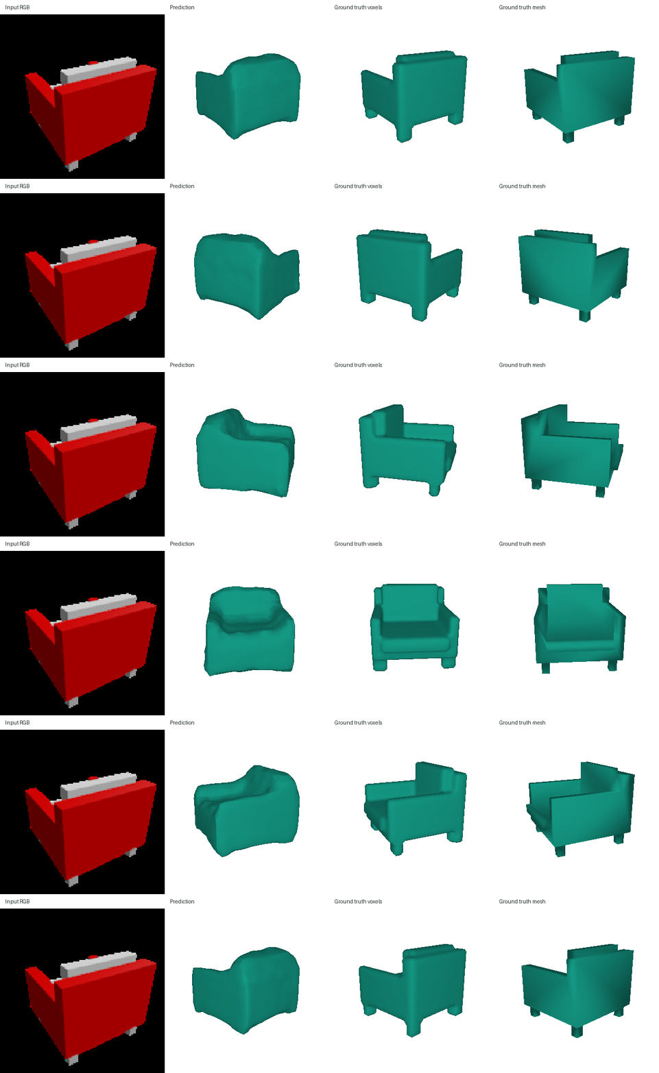
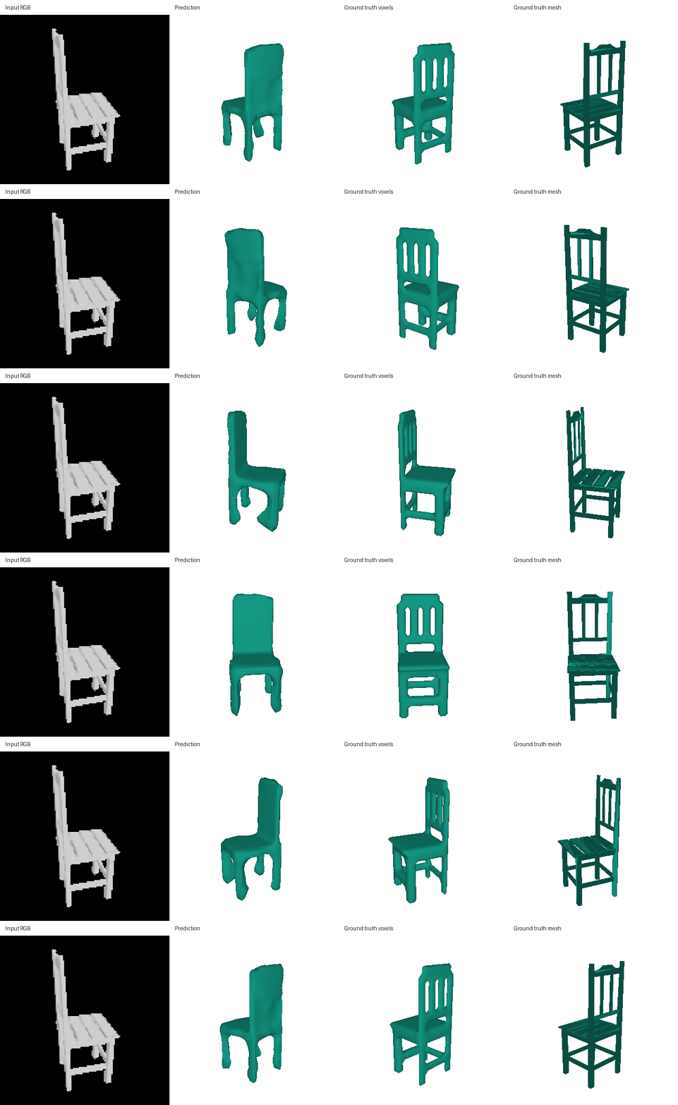
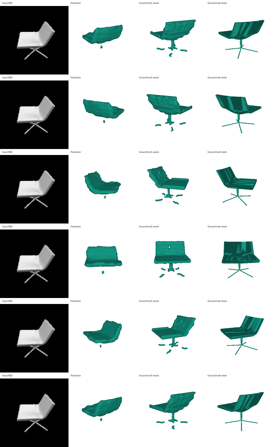
The model fills the openings in chair 339’s back and misses chair 677’s thin base. The target voxel grid also breaks the thin base, so grid resolution is part of the limitation.
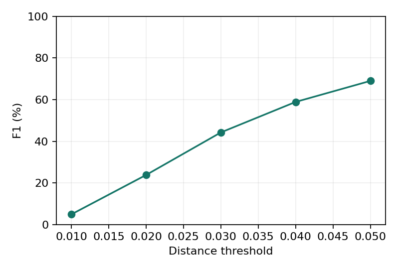
Image to point cloud
The decoder is an MLP with three hidden layers of width 1,024. It predicts 1,000 XYZ points and is trained with the symmetric Chamfer loss.
The final model trains for 8,890 updates. Test F1@0.05: 80.64.
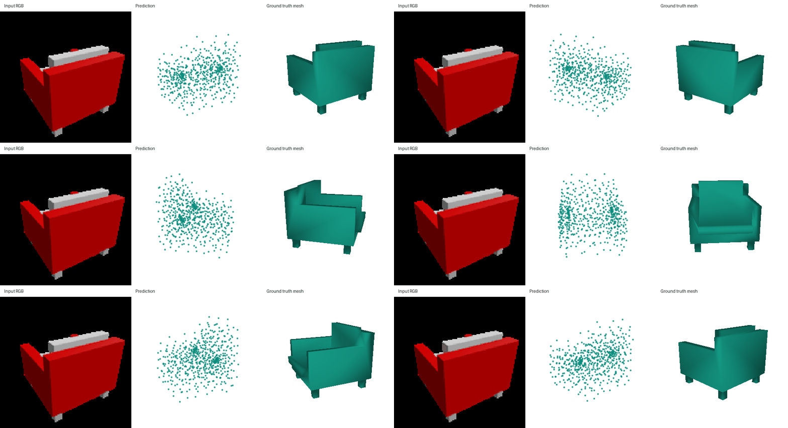
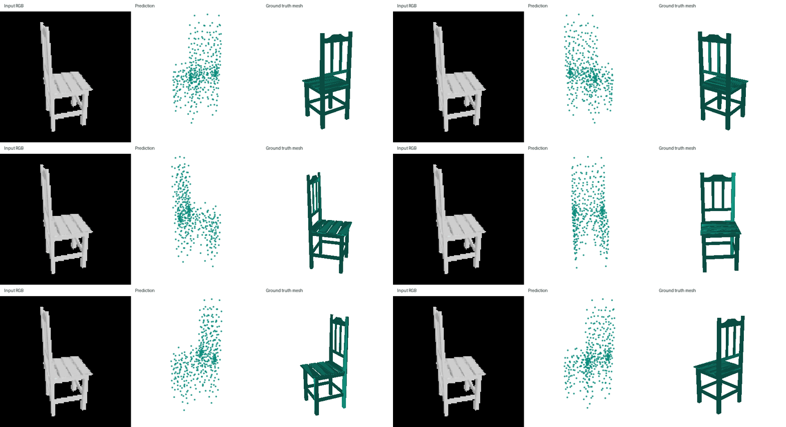
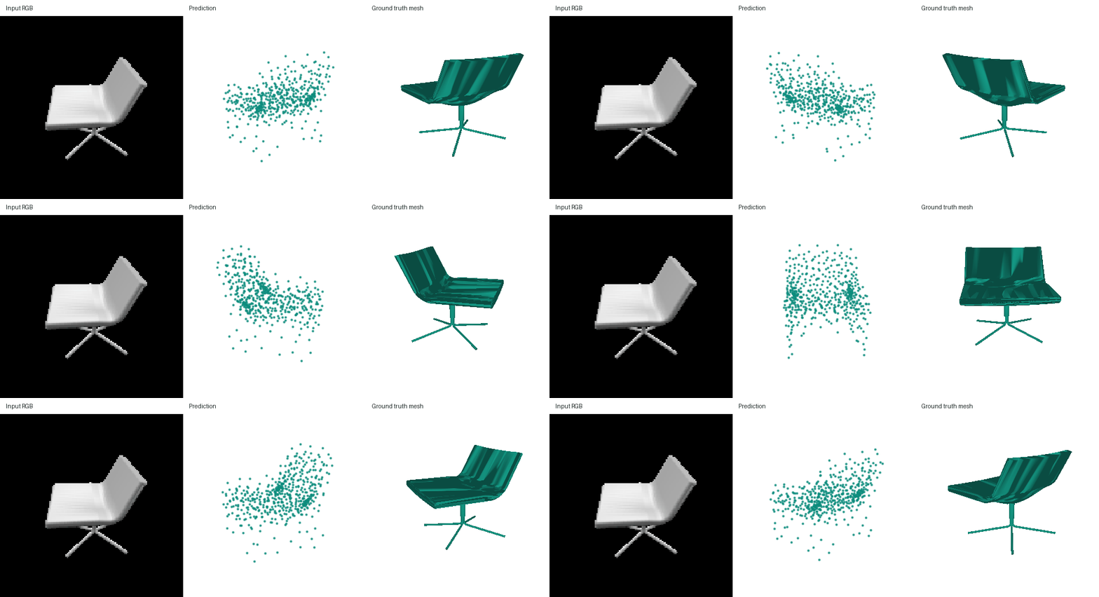
The point clouds remain noisy. A point can lie almost 0.05 away from the target and still count as correct, so this score can be high even when thin bars and legs are poorly resolved.
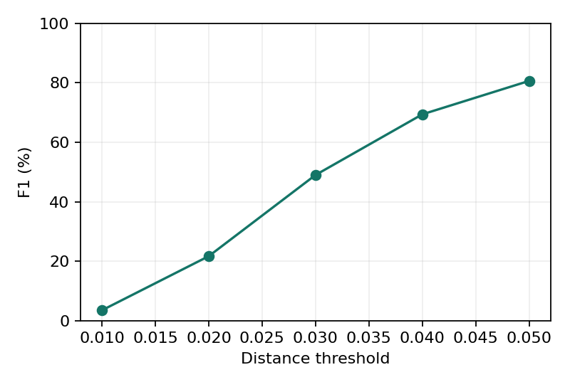
Image to mesh
We use eight generic square mesh patches with 1,024 vertices in total. Each square has an 8 × 16 vertex grid; the patches start at evenly spaced depths. A shared projection maps the image feature to 128 dimensions. Each patch has its own MLP with three hidden layers of width 256, conditioned on this code and the template coordinates, and predicts vertex offsets. The initial connectivity stays fixed.
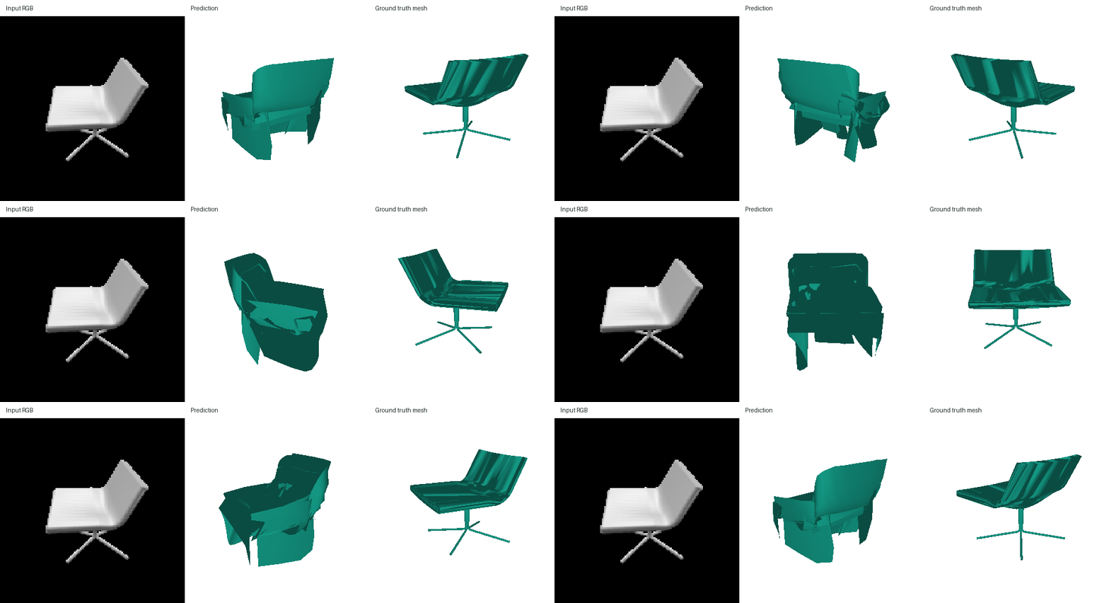
We train with symmetric Chamfer loss between 1,000 points sampled from the predicted triangles and 1,000 target surface points, without additional mesh penalties. Q2.4 compares these choices on validation objects.
The final model trains for 6,667 updates. Test F1@0.05: 75.55.
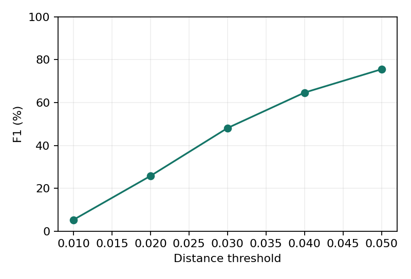
| Representation | Test F1@0.05 |
|---|---|
| Voxel grid | 69.00 |
| Point cloud | 80.64 |
| Mesh | 75.55 |
Points can move independently to cover thin or disconnected regions. Voxels lose detail at 32³ resolution. The mesh represents connected surface patches, but gaps and overlaps can remain between them. A high F1 does not guarantee correct topology or sharp details.
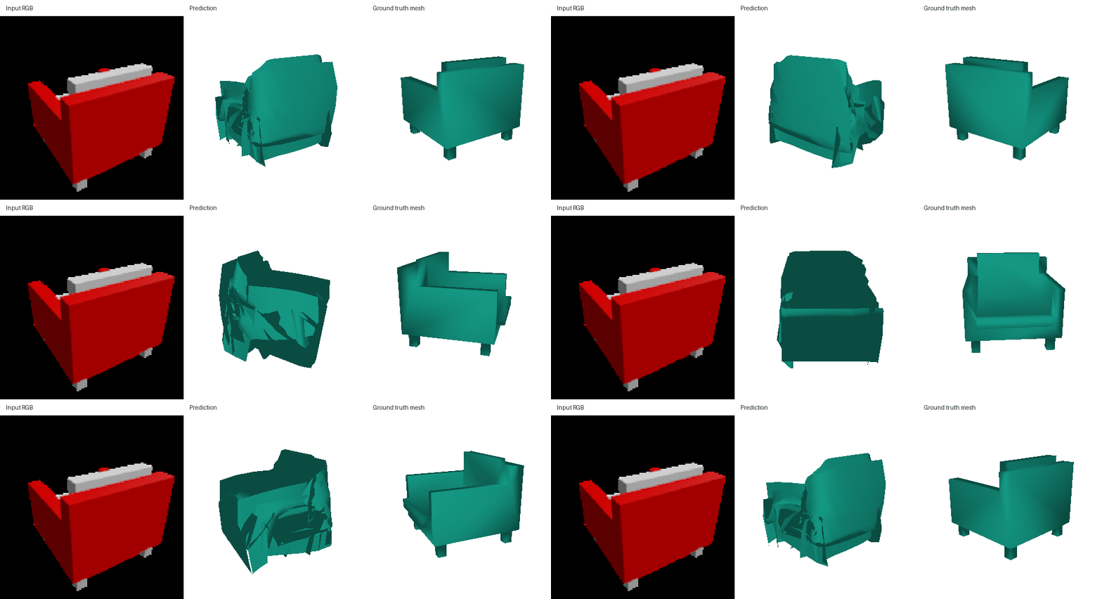
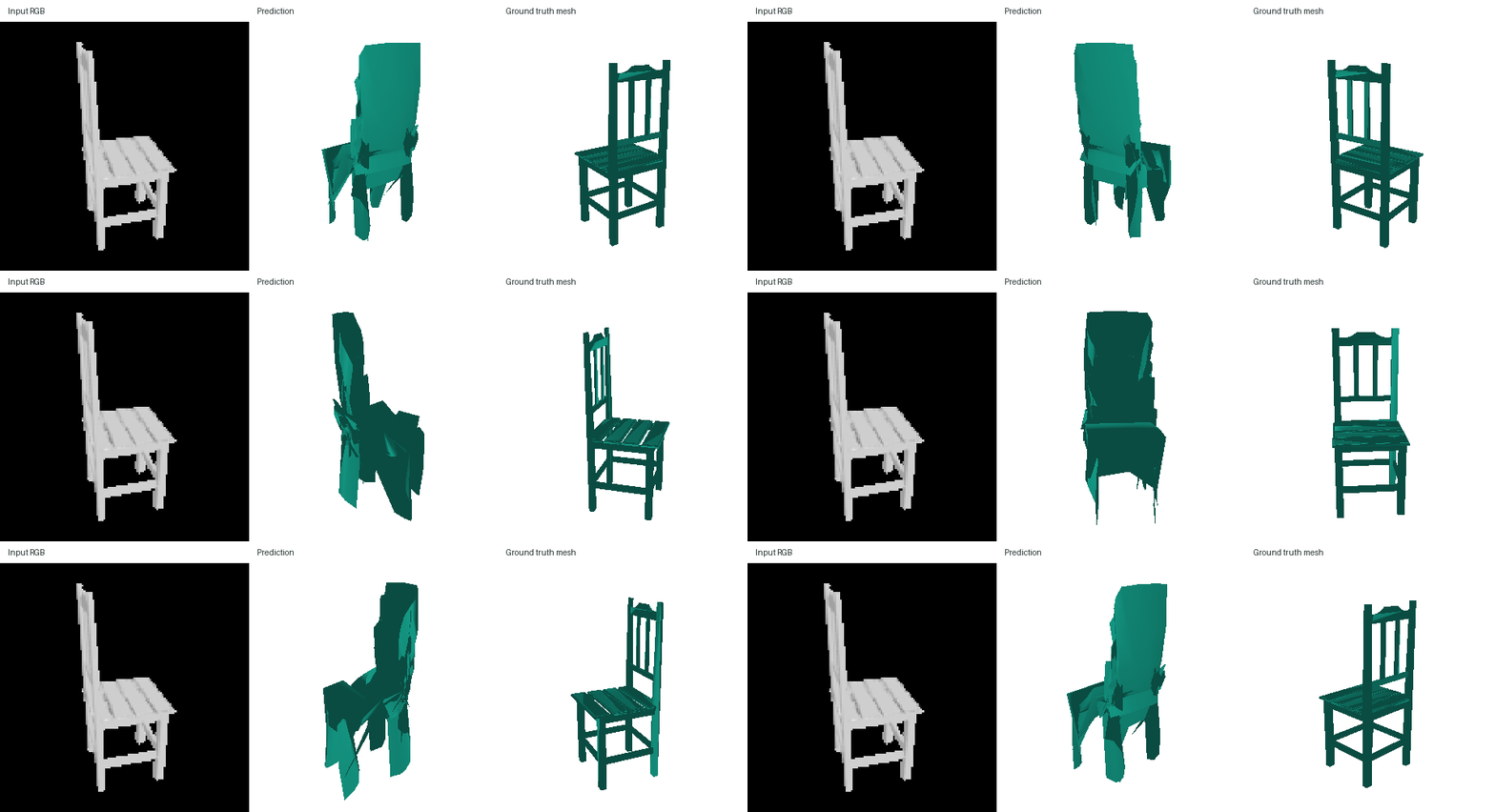
The model forms broad seat and back surfaces, but still misses important details. Chair 339 has a filled back despite its high F1, and chair 677 has broad panels in place of the thin pedestal base. Chair 0 also has fragmented side surfaces.
Mesh initialization and decoder ablations
Every run below uses 6,000 updates, batch size 32, seed 4825, and the same 5,490 training and 610 validation chairs. All ten training views are used. Scores use the final checkpoint and the first listed validation view. Test objects are excluded from model selection.
1. Initial shape and resolution
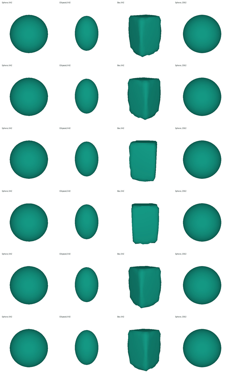
We first compare a sphere, ellipsoid, and box with the same 642 vertices and connectivity. The sphere has radius 0.4; the ellipsoid semi-axes and box half-extents are (0.25, 0.38, 0.25). The loss is surface Chamfer plus Laplacian, edge, and normal-consistency terms with weights 0.02, 0.5, and 0.01.
| Initial shape | Vertices | Validation F1@0.05 |
|---|---|---|
| Sphere | 642 | 70.53 |
| Ellipsoid | 642 | 70.56 |
| Box | 642 | 70.57 |
| Sphere | 2562 | 73.08 |
The three coarse shapes are nearly tied. The denser sphere improves F1, but still has stretched surfaces. A different initial shape alone is insufficient.
2. Generic closed components
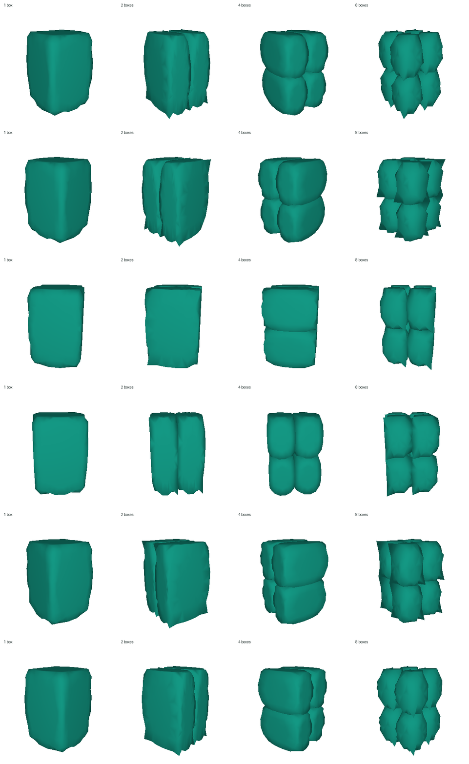
We carry the box forward and compare 1, 2, 4, and 8 components in a regular grid. All models have 648 vertices in total, the same overall bounds, and identical decoder sizes and initial weights. No component is assigned a chair part. We use 648 so the vertex count divides equally across the tested component counts.
| Components | Validation F1@0.05 |
|---|---|
| 1 | 70.72 |
| 2 | 70.44 |
| 4 | 70.11 |
| 8 | 69.70 |
Adding closed components reduces F1 in this comparison. It does not fix the reconstruction problem.
3. Continuous deformation and combinations
AtlasNet generates surfaces with coordinate-conditioned networks. We test this idea by feeding each template vertex, its component center, and a 128-dimensional image code to a shared MLP with three hidden layers of width 256. The output is a vertex offset. Nearby template coordinates now pass through the same function.
At 648 vertices, this decoder scores 68.85. Replacing surface-sampled Chamfer with vertex Chamfer scores 67.71; we retain surface sampling. Vertex Chamfer is used in Pixel2Mesh, but does not help this decoder in our comparison.
We then test denser boxes with 2,592 total vertices. Regularization ×0.1 scales all three weights above by one tenth; ×1 keeps them unchanged. The transfer experiment initializes ResNet18 from our point model trained for 8,000 updates on the same training objects, then fine-tunes it. This adds pretraining compute.
| Model change | Validation F1@0.05 |
|---|---|
| Independent vertex offsets | 73.48 |
| Continuous field, regularization ×1 | 70.40 |
| Continuous field, regularization ×0.1 | 72.62 |
| Continuous field, no regularization | 72.89 |
| Two closed components, field, ×0.1 | 72.30 |
| Point-trained encoder, field, ×0.1 | 72.27 |
Weaker penalties help the continuous decoder, but none of these combinations beats direct vertex offsets. Encoder transfer and two closed components do not improve it.
4. Open patches and independent networks
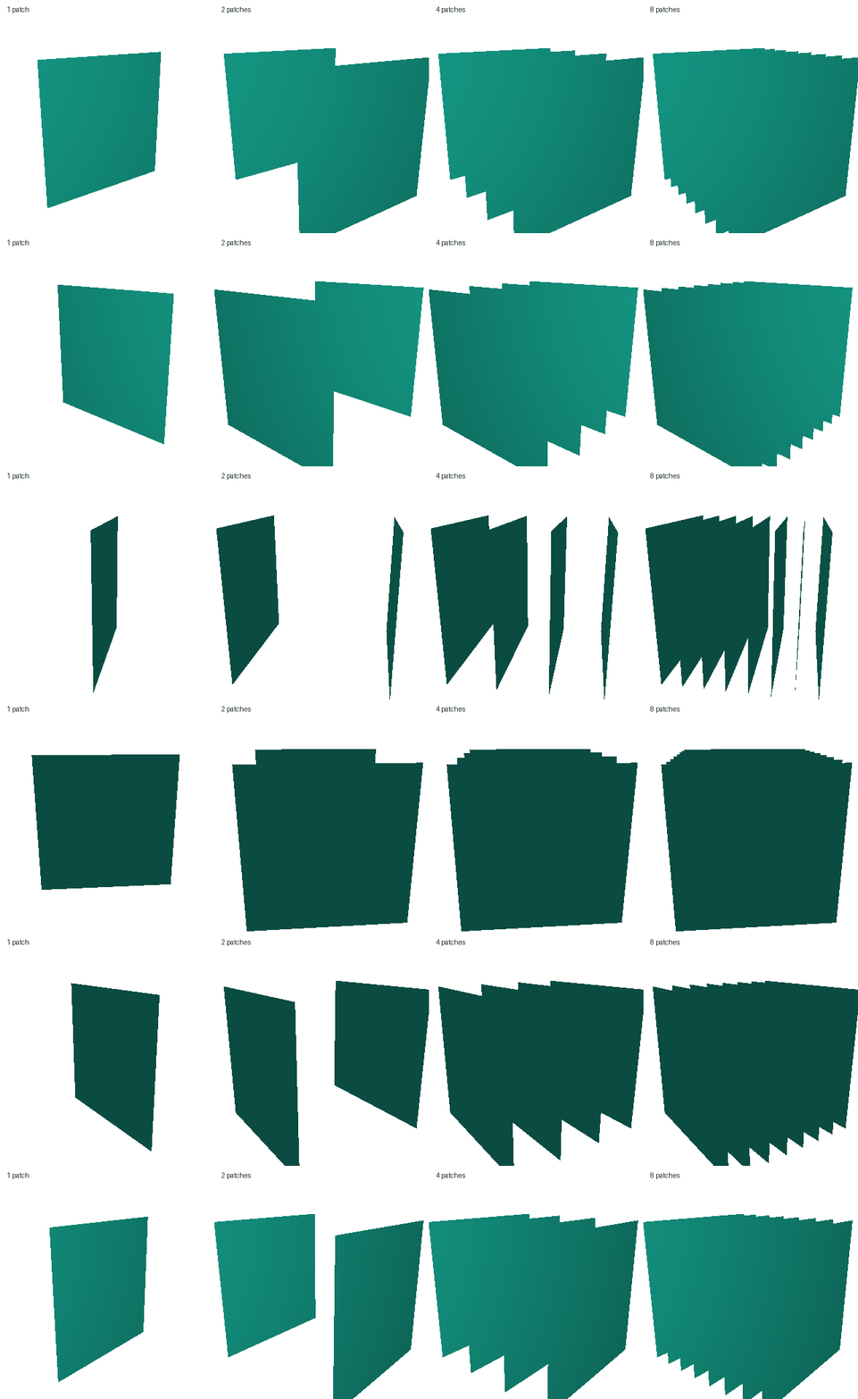
AtlasNet also uses open square patches. We test 1, 2, 4, and 8 parallel square templates, keeping 1,024 total vertices and the same shared decoder. The patches start at evenly spaced depths and have no assigned semantic roles. These runs use surface Chamfer without extra mesh penalties. A closed box with the same vertex count and decoder provides a topology comparison.
| Template and decoder | Components | Validation F1@0.05 |
|---|---|---|
| Closed box; shared network | 1 | 72.34 |
| Open squares; shared network | 1 | 70.91 |
| Open squares; shared network | 2 | 72.75 |
| Open squares; shared network | 4 | 73.90 |
| Open squares; shared network | 8 | 74.47 |
| Open squares; shared network + encoder transfer | 8 | 73.65 |
| Open squares; independent networks | 1 | 71.39 |
| Open squares; independent networks | 4 | 73.87 |
| Open squares; independent networks | 8 | 74.80 |
| Open squares; independent networks, direct XYZ | 8 | 74.39 |
Independent networks give each patch its own MLP, following AtlasNet’s multi-chart design. The shared decoder has 0.23 million parameters; independent decoders have 0.23, 0.73, and 1.40 million parameters for 1, 4, and 8 patches. Their gains therefore include increased decoder capacity.
Eight independent patches score 74.80, the highest validation F1 in this study. Direct XYZ prediction scores 74.39 and does not improve it. We select the eight-patch offset model. Compared with vertex offsets, its surfaces are less fragmented, but overlaps and missing thin bars remain.
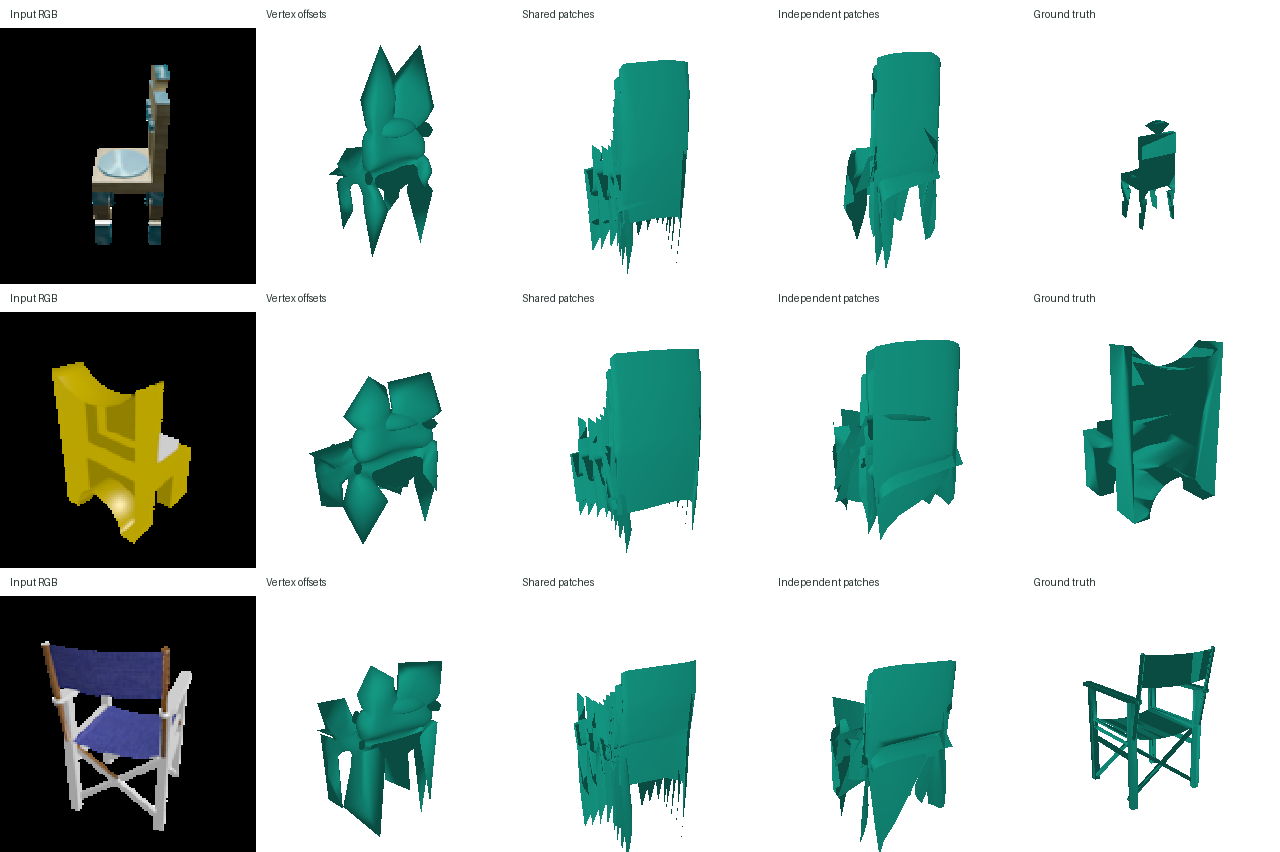
We select the highest validation F1 after 6,000 updates, then refit the chosen configuration on all 6,100 training chairs for 6,667 updates. This preserves the number of passes through the image–shape pairs.
Where do the models miss the surface?
We test whether coverage is worse near changes in surface direction. For each test mesh, we sample 8,192 surface points and measure normal variation among up to 32 neighbors within distance 0.035. Opposite parallel normals count as aligned. We compare the lowest and highest quarters of normal variation within each chair.
Recall is the percentage of target points within 0.05 of a predicted point. We average each region’s recall across all 678 test chairs. The control replaces the prediction with 1,000 points sampled from the correct mesh, to show how much sparse sampling alone affects coverage.
| Prediction | Low normal variation: recall (%) | High normal variation: recall (%) |
|---|---|---|
| GT sampling control | 99.66 | 99.77 |
| Voxel grid | 71.69 | 63.14 |
| Point cloud | 83.22 | 78.99 |
| Mesh | 78.85 | 74.66 |
Coverage is lower in regions with changing normals for all three models. Recall drops by 8.56 points for voxels, 4.23 for points, and 4.19 for meshes. The ground-truth sampling control does not show this drop. This supports more reliable coverage of locally planar regions.
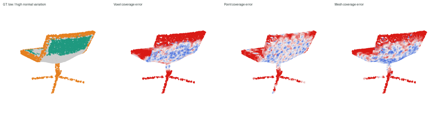
This measures missed surface regions. It does not measure floating predicted points, which are penalized by precision in the F1 score. It also does not establish that training reached a local minimum.
Implicit network
The implicit decoder takes an image feature and a 3D query point and predicts occupancy. It uses four residual MLP blocks of width 256, with the image feature added at each block. The coordinate input includes sine and cosine features at four frequencies. We train with 2,048 uniformly sampled cells per image and the same occupancy loss as the voxel decoder.
At evaluation, we query all 32³ cell centers in (−1, 1)³ and extract the surface at probability 0.6. The model trains for 22,223 updates. Test F1@0.05: 70.05.
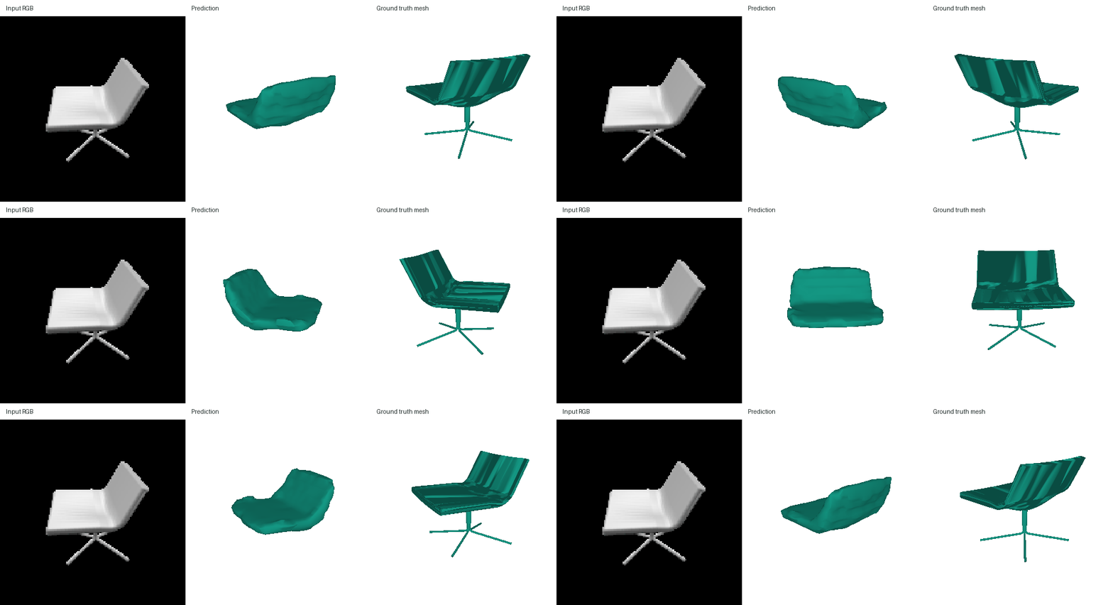
The coordinate network produces a continuous occupancy function, but supervision is still a 32³ grid. It cannot recover fine geometry that those targets do not contain.
Parametric network
Eight MLPs map 2D points from a square, together with the image feature, to 3D. We sample 125 points per patch and train the resulting 1,000-point cloud with Chamfer loss. Evaluation uses fixed, evenly distributed points over each square.
Test F1@0.05: 78.84. For the surface display below, we evaluate each learned map on a 32 × 32 grid and connect adjacent grid points.
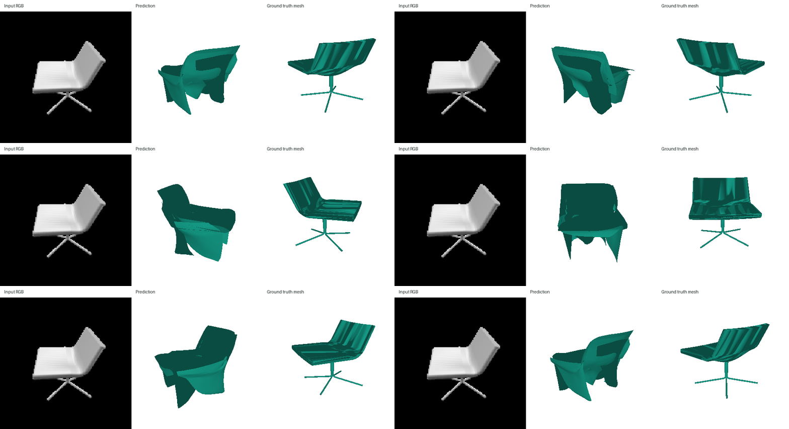
The patches can represent separate parts, but their boundaries are not constrained to meet. This can leave seams, overlaps, and gaps.
Training on three classes
We train the same point decoder on 6,100 chairs, 3,146 cars, and 3,640 planes. Both models use the same batch size and 8,890 updates. The larger dataset therefore receives fewer passes per object.
| Training data | Chair test F1@0.05 |
|---|---|
| Chairs | 80.64 |
| Chairs, cars, and planes | 80.63 |
Chair F1 decreases by 0.01 points when adding the other classes. The three-class model scores 93.56 on cars and 96.46 on planes.

The chair scores are effectively unchanged at this training budget. Adding cars and planes lets one model cover all three categories, but it does not improve chair reconstruction overall. The example still misses the thin pedestal base in both predictions.