

Loss Function: Binary Cross-Entropy with Logits
Loss Function: Chamfer Distance (took the mean, not sum of the minimum distances).
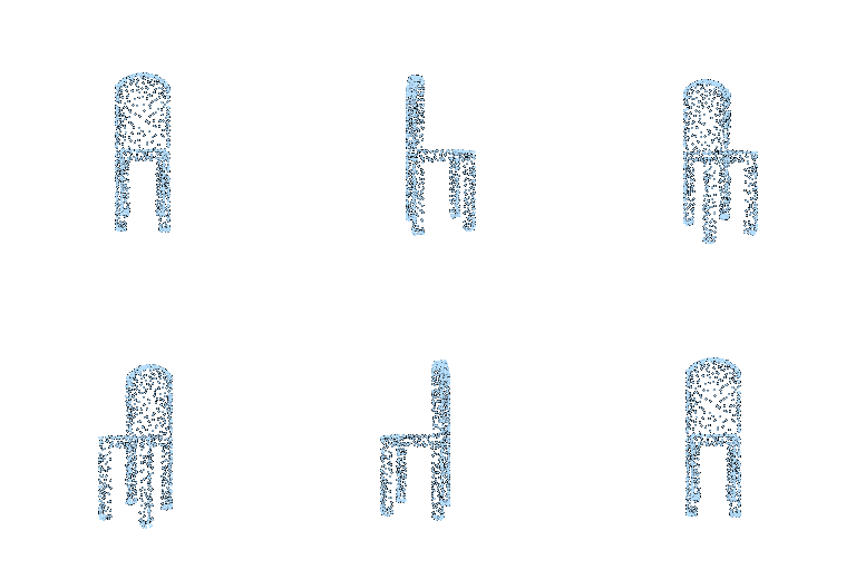
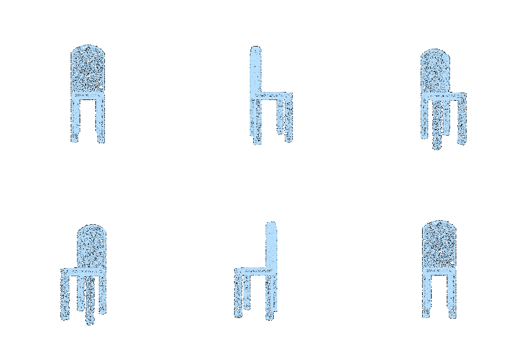
Loss Function: Combination of Chamfer distance with mesh Laplacian smoothing
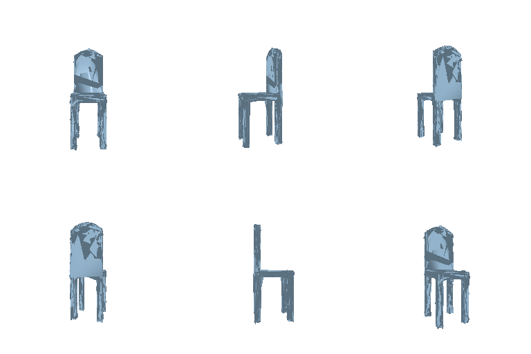

All models use the same pretrained image feature vector with --load_feat but decoder is designed differently.
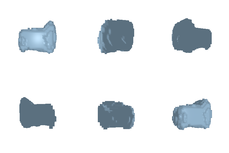
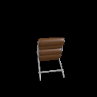
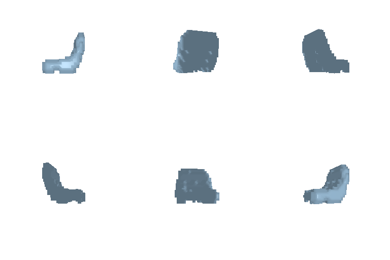
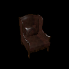
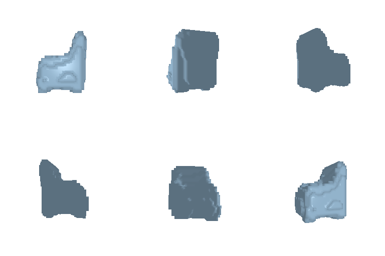
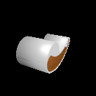
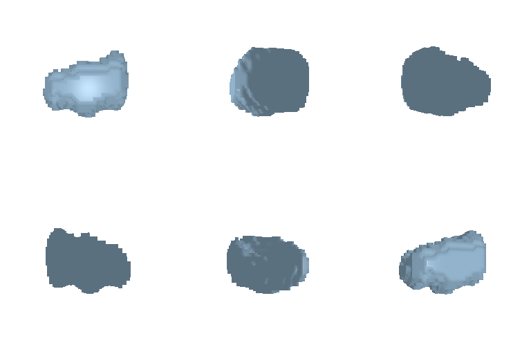
The voxel decoder uses a fully connected layer followed by 3D transposed-convolution blocks that progressively upsample the image feature into a 32×32×32 occupancy grid. Same loss function as above is used for training.
Avg F1@0.05: 61.560
| Input Image | Ground Truth | Prediction |
|---|---|---|
 |
 |
 |
 |
 |
 |
 |
 |
 |
 |
 |
 |
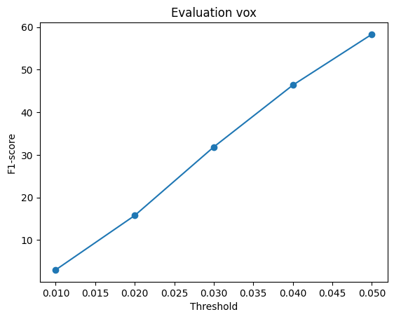
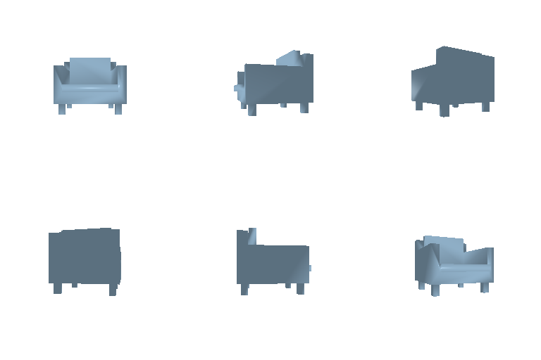
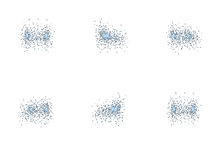
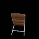
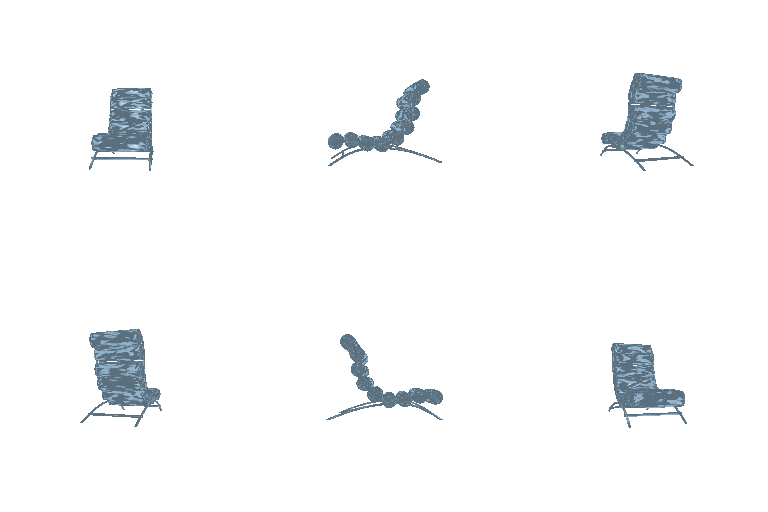
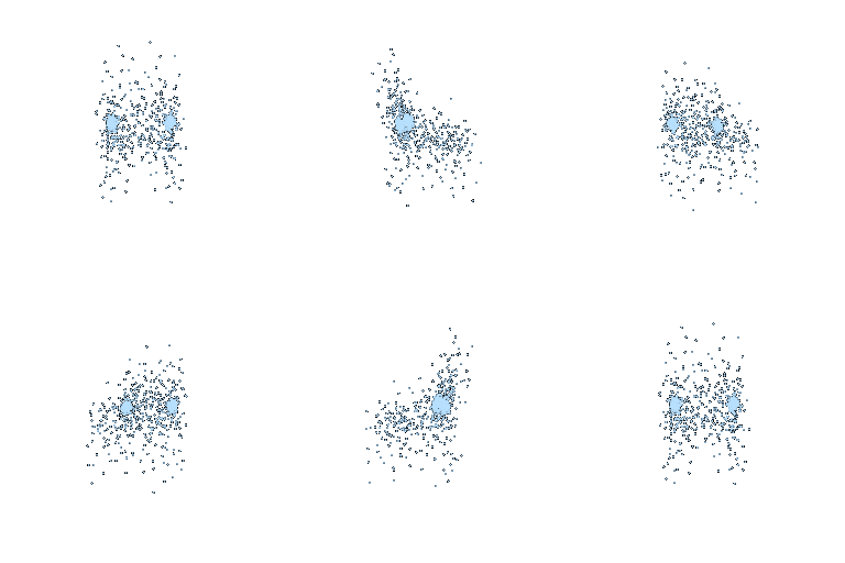
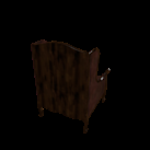
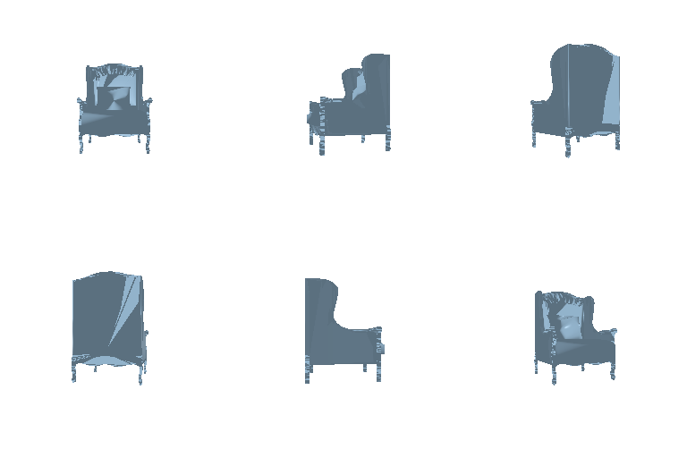
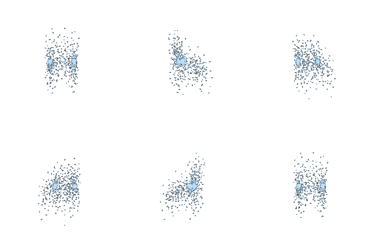
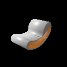
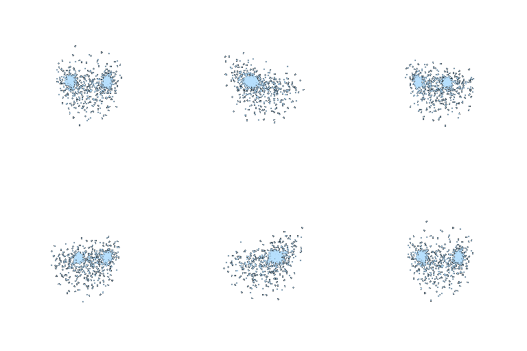
The point decoder maps the 512-dimensional image feature through an MLP and directly predicts n_points × 3 coordinates. Same loss function as above is used for training.
Avg F1@0.05: 73.216
| Input Image | Ground Truth | Prediction |
|---|---|---|
 |
 |
 |
 |
 |
 |
 |
 |
 |
 |
 |
 |
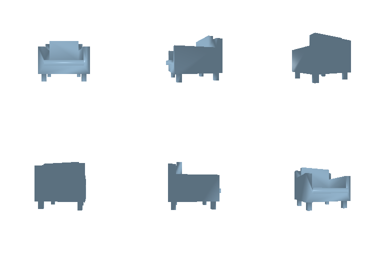
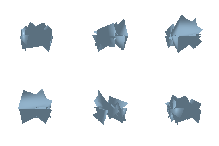
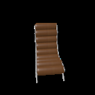
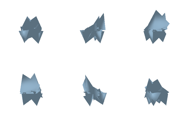
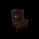
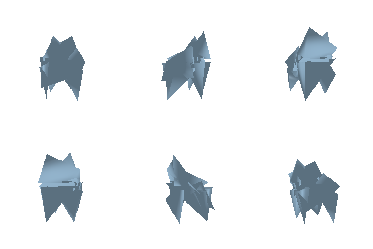
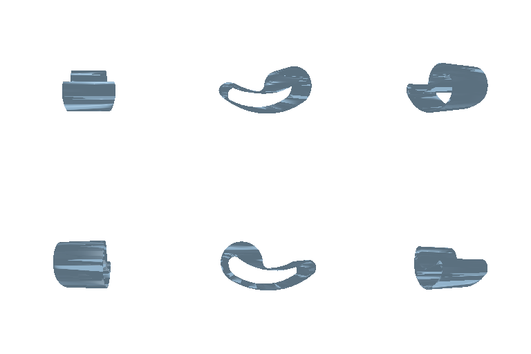
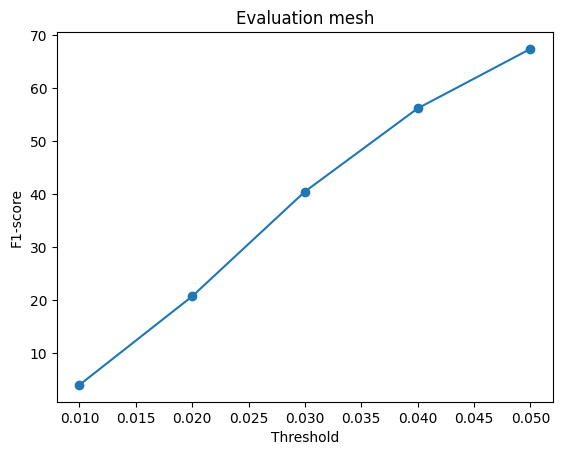
The mesh model begins with an icosphere template and predicts an XYZ displacement for every template vertex with the decoder which maps the 512-dimensional image feature through an MLP. Same loss function as above is used for training.
Avg F1@0.05: 67.457
| Input Image | Ground Truth | Prediction |
|---|---|---|
 |
 |
 |
 |
 |
 |
 |
 |
 |
 |
 |
 |
| Representation | Avg F1@0.05 | Main advantage | Main limitation |
|---|---|---|---|
| Voxel | 61.560 | Stable volumetric occupancy | Resolution limits thin details |
| Point cloud | 73.216 | Flexible surface coverage | No explicit connectivity |
| Mesh | 67.457 | Connected, renderable surface | Fixed topology and harder optimization |
Intuitive Analysis: Point clouds win by freely placing dots anywhere, meshes struggle to stretch a solid skin over complex shapes, and voxels score lowest because chunky blocks lose fine details.
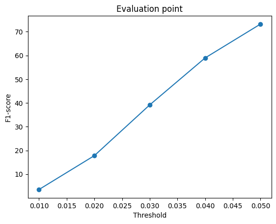
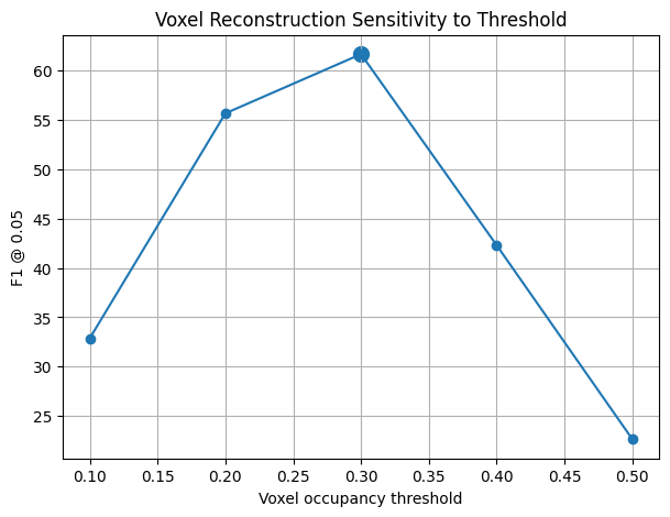
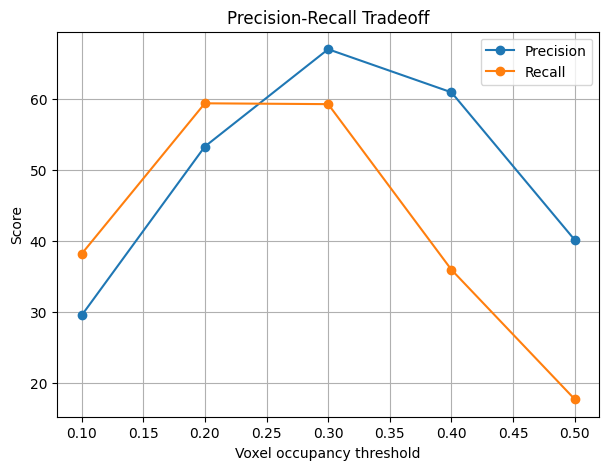
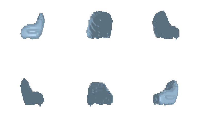
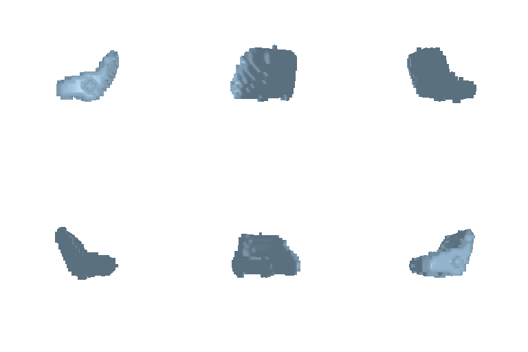
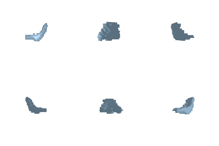
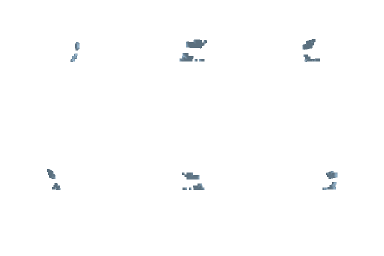
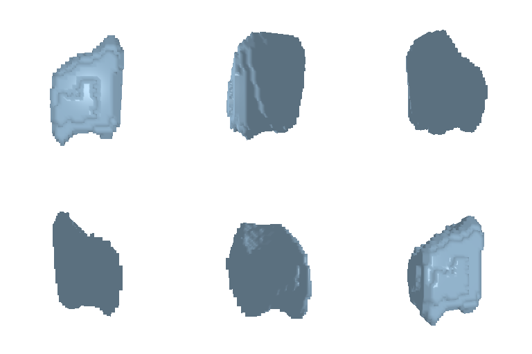
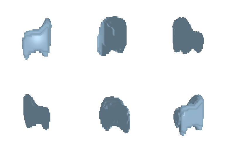
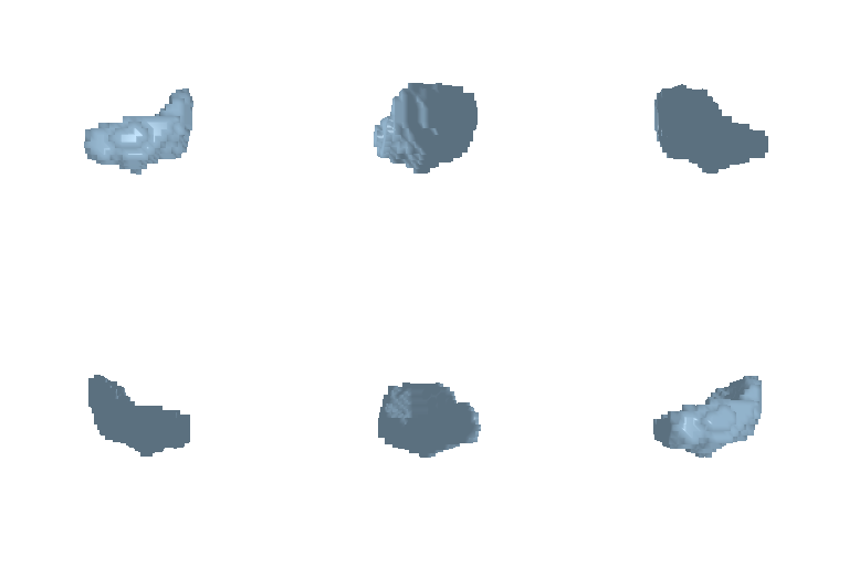
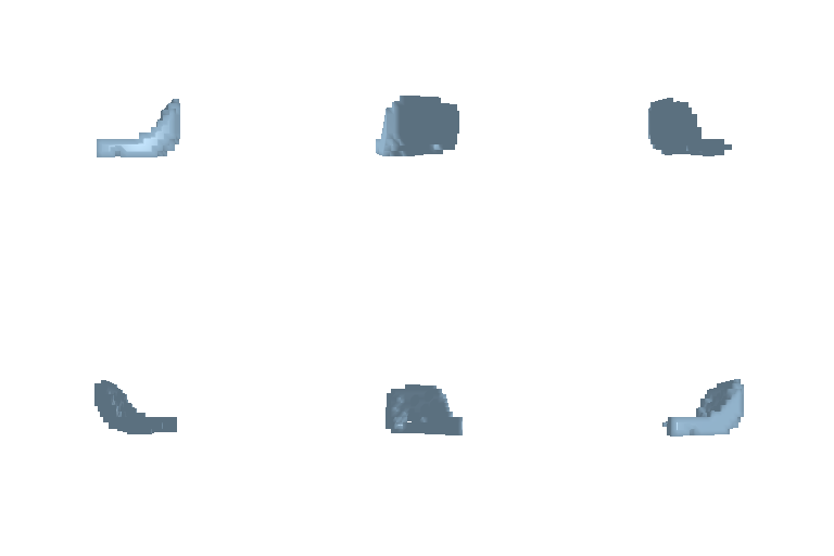
I evaluated the voxel reconstruction model across different occupancy thresholds to analyze the tradeoff between precision and recall. As the threshold increases, the F1 score peaks at 0.30 before sharply declining. The precision-recall curves demonstrate that a threshold of 0.3 maximizes precision, while higher thresholds cause both metrics to drop, and lower thresholds favor recall.
| Threshold | Precision | Recall | F1@0.05 |
|---|---|---|---|
| 0.1 | 29.551 | 38.205 | 32.866 |
| 0.2 | 53.328 | 59.409 | 55.680 |
| 0.3 | 67.020 | 59.293 | 61.684 |
| 0.4 | 60.953 | 35.991 | 42.306 |
| 0.5 | 40.182 | 17.770 | 22.646 |
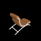
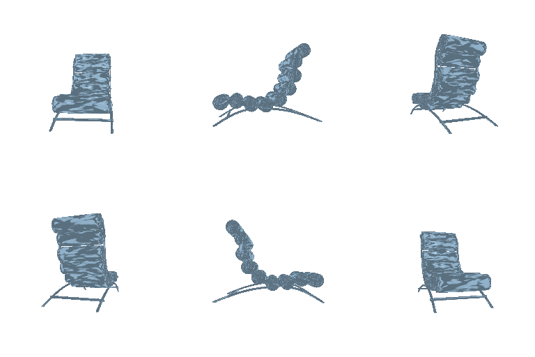
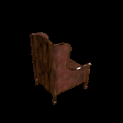
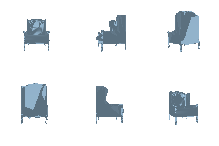
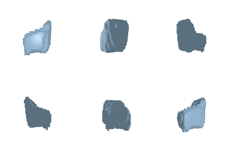
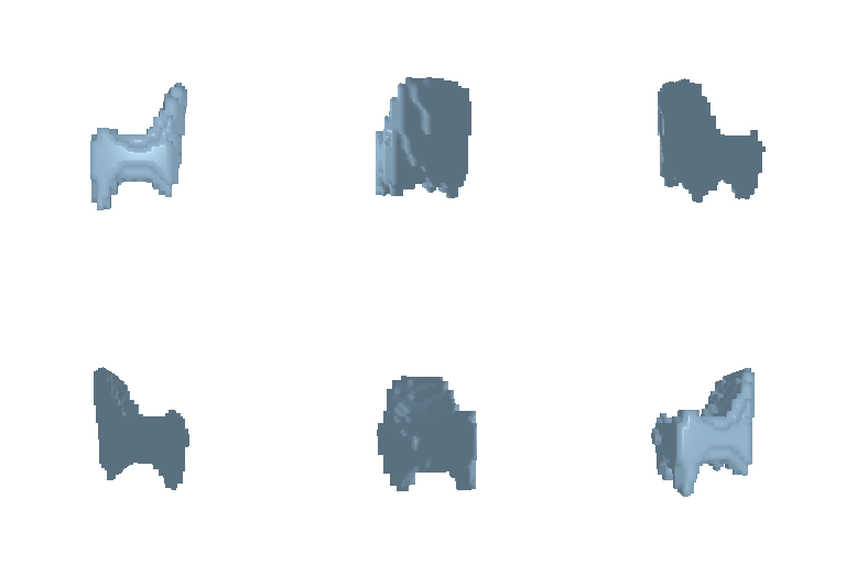
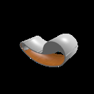
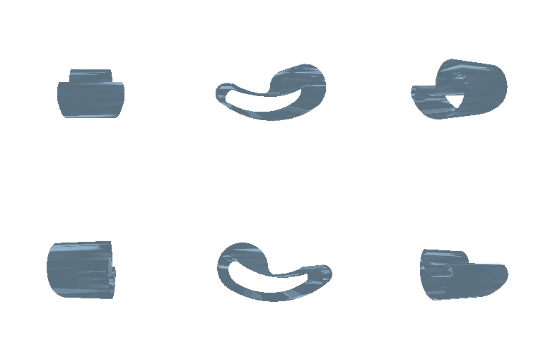
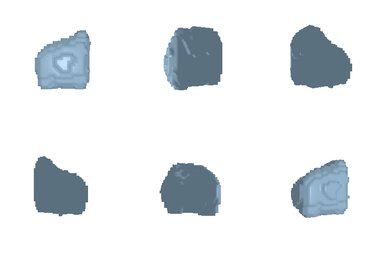
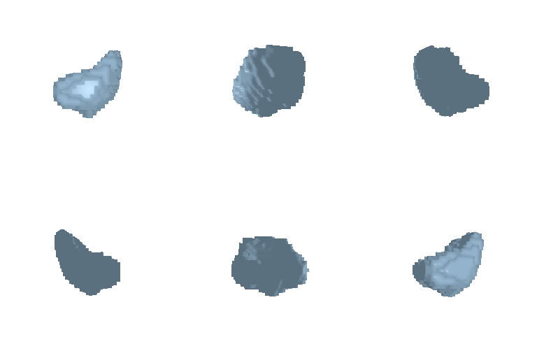
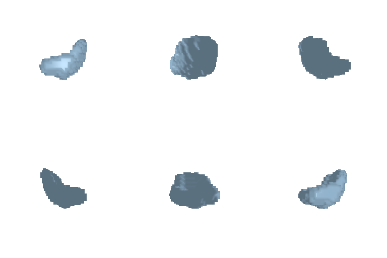
The table below visualizes how the predicted voxel geometry changes as the binarization threshold increases. Lower thresholds produce thicker, blob-like structures, while higher thresholds erode thin details entirely.
| Input Image | Ground Truth | Threshold = 0.1 | Threshold = 0.2 | Threshold = 0.3 | Threshold = 0.4 | Threshold = 0.5 |
|---|---|---|---|---|---|---|
 |
 |
 |
 |
 |
 |
Empty Voxel (No voxels > 0.5) |
 |
 |
 |
 |
 |
 |
 |
 |
 |
 |
 |
 |
 |
 |
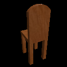
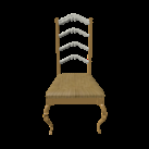
To inspect more than just final evaluation scores, I implemented post-hoc visualization techniques to understand how the network maps 2D visual evidence to 3D voxel geometry.
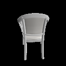
Specifically, I generated occlusion sensitivity heatmaps. By systematically sliding an 8×8 constant-color patch across the input image and measuring the mean absolute difference in the resulting voxel probabilities, we can visualize which image regions the network relies on most. Red/warmer areas indicate regions where occluding the image drastically changes the 3D output.
| Input Image | Occlusion Heatmap | Ground Truth | Prediction |
|---|---|---|---|
 |
 |
 |
 |
 |
 |
 |
 |
 |
 |
 |
 |
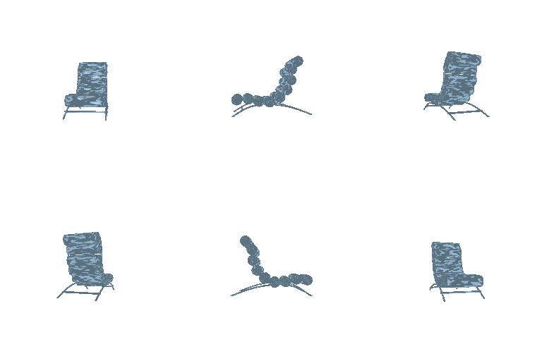
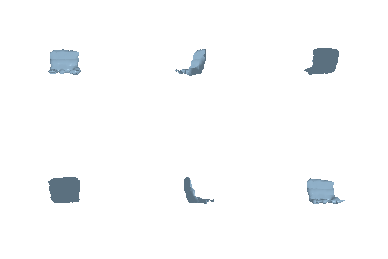
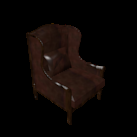
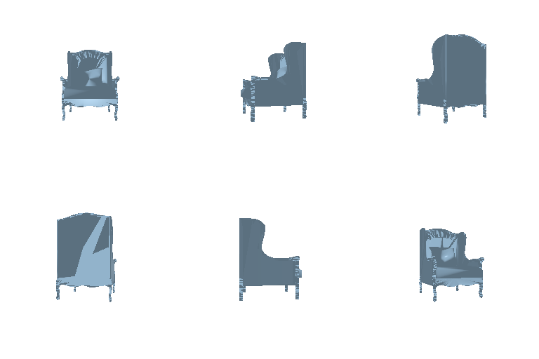
Instead of using 3D convolutions, this implicit decoder models shape by mapping spatial coordinates to occupancy probabilities using an MLP. The function is defined as:
where \(\mathbf{x} = (x,y,z)\) is a spatial coordinate, \(\mathbf{z}\) is the 512-dimensional image feature, and \(o\) is the occupancy logit. To help the network learn high-frequency geometric details, the 3D coordinates are first passed through a sinusoidal positional encoding \(\gamma(\mathbf{x})\) across 6 frequency bands.
While implicit networks are theoretically continuous, my implementation optimizes this for a voxel-based pipeline. During initialization, the network pre-computes a uniform 32³ coordinate grid spanning \([-1,1]^3\). In the forward pass, the MLP evaluates these 32,768 fixed points simultaneously and reshapes the output directly into a 32³ voxel tensor. This allows the model to leverage coordinate-conditioned MLP layers while still training end-to-end with the standard explicit voxel loss.
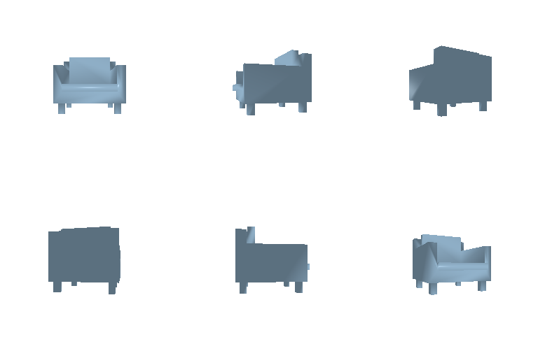
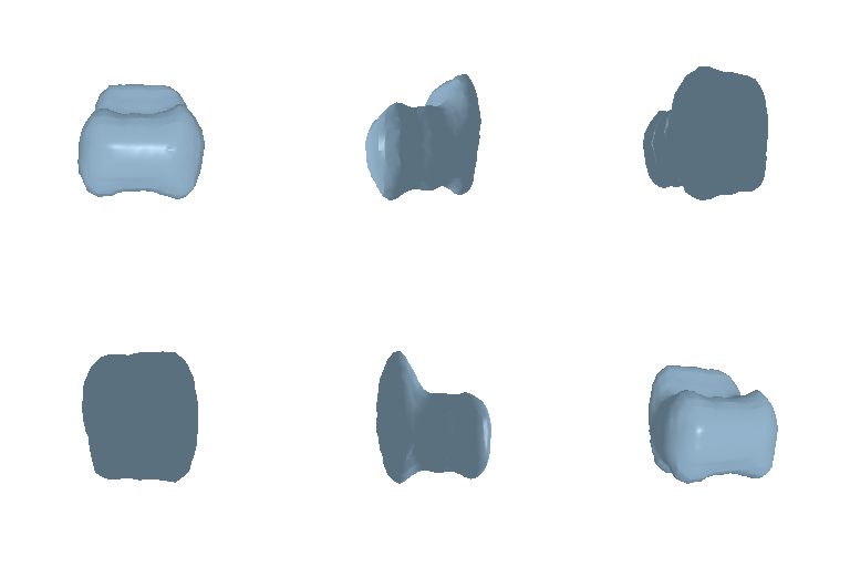
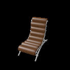
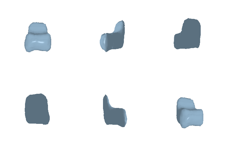
Avg F1@0.05: 42.436
| Input Image | Ground Truth | Prediction |
|---|---|---|
 |
 |
 |
 |
 |
 |
 |
 |
 |
 |
 |
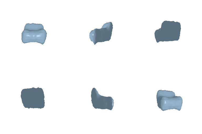 |
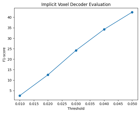
Analysis: The implicit formulation successfully learns to map continuous 3D coordinates to occupancy probabilities, scoring an Avg F1@0.05 of 42.436. While it offers a flexible, memory-efficient view of occupancy (avoiding the \(O(N^3)\) memory scaling of explicit voxel grids during training), it scored lower than the explicit voxel baseline (61.560). This performance gap highlights that implicit networks can be more challenging to optimize and are highly sensitive to hyperparameters such as coordinate normalizations, the number of positional encoding frequencies, and the density of points sampled during training.
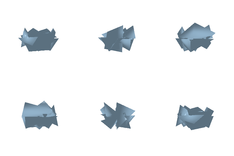
The parametric decoder maps a continuous 2D domain into 3D space. Instead of predicting all 3D coordinates at once, it learns a function:
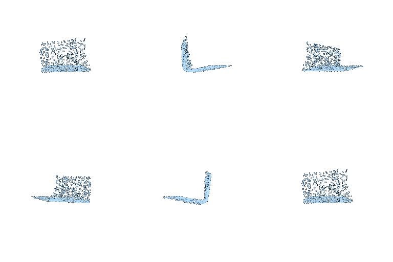
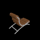
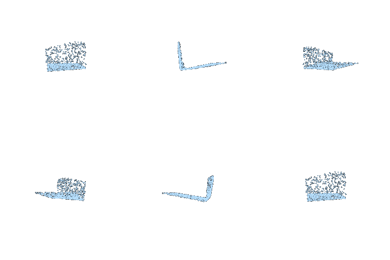
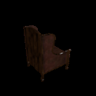
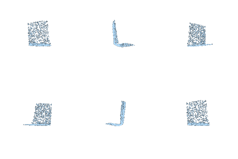
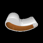
where \((u,v)\) is a 2D coordinate and \(\mathbf{z}\) is the image feature. In my implementation, I randomly sampled 2D points in the range \([-1, 1]^2\). Each \((u,v)\) coordinate is concatenated with the 512-dimensional image feature to form a 514-dimensional vector. An MLP then processes this vector to predict a specific 3D point location. The model is trained using symmetric Chamfer loss against points sampled from the ground-truth mesh.
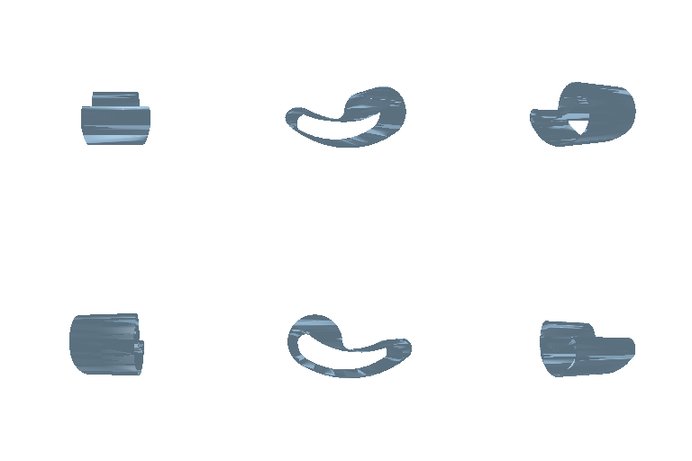
Avg F1@0.05: 46.117
| Input Image | Ground Truth | Prediction |
|---|---|---|
 |
 |
 |
 |
 |
 |
 |
 |
 |
 |
 |
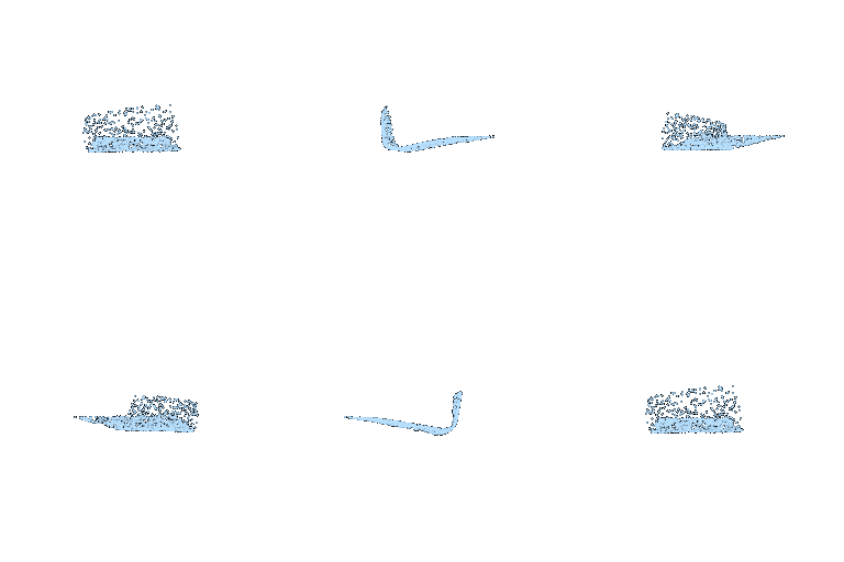 |
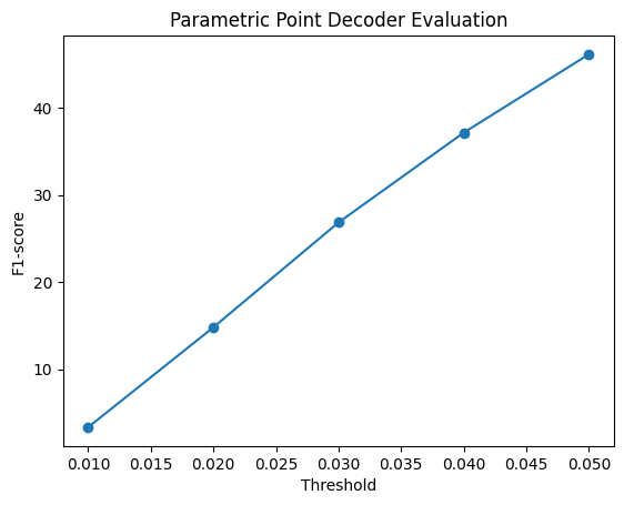
Analysis: Unlike the standard point decoder that acts as an unconstrained coordinate generator, the parametric network ties every predicted 3D point to a specific 2D domain origin. The model achieved an Avg F1@0.05 of 46.117, which is notably lower than the direct point-cloud decoder’s 73.216. This performance gap makes sense geometrically: the parametric model is essentially trying to fold and stretch a single 2D sheet of paper to cover complex chair topologies (which often feature holes, disconnected legs, and sharp angles). While the 2D domain provides a continuous structural organization, a single patch struggles to represent the multi-chart surface of a chair.
These experiments demonstrate that the choice of 3D representation fundamentally alters both the learning dynamics and the resulting geometry. Explicit voxels are stable and capture solid occupancy well, but suffer from resolution bottlenecks. Explicit point clouds achieve the highest distance-based metrics by freely scattering points over surfaces, but fail to provide continuous topology. Explicit meshes strike a balance by providing renderable, connected surfaces, though they are heavily constrained by their initial template topology.
On the other hand, the implicit model offers an elegant, resolution-free view of continuous occupancy but proved sensitive to hyperparameter tuning and class imbalance. Finally, the parametric model added an interesting structural mapping by anchoring points to a 2D domain, illustrating that while topological constraints can help organize data, forcing complex multi-part objects into a single continuous patch is an extremely difficult optimization problem.