Assignment 3: Volume Rendering, NeRF, and 3D Gaussian Splatting
Ashutosh Panda · CMU · Fall 2026
This report presents the implementation and results for differentiable volume rendering, NeRF, and 3D Gaussian splatting. View-dependent NeRF (4.1) and spherical harmonics (7.1) are the selected extensions. VolSDF (4.3) and harder-scene training (7.2) are additional experiments.
1. Differentiable Volume Rendering
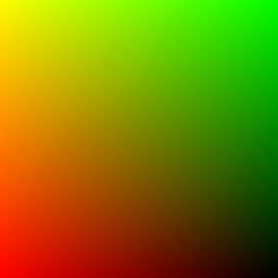
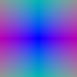
1.3 Ray sampling
Pixel coordinates are generated in [−1, 1] and unprojected from camera NDC into world coordinates. Ray origins are the camera center, and directions are normalized vectors toward the unprojected points.
1.4 Point sampling
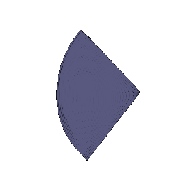
For each ray, I uniformly sample distances between the near and far bounds and compute sample positions as xᵢ = o + tᵢd. The sampled positions and distances are stored in the RayBundle.
1.5 Volume rendering
I compute opacity from density and segment length, then use exclusive transmittance to obtain per-sample weights. Weighted sums produce RGB and depth. The first sample has transmittance 1.
αᵢ = 1 − exp(−σᵢ Δtᵢ)
Tᵢ = exp(−Σⱼ<ᵢ σⱼ Δtⱼ)
wᵢ = Tᵢ αᵢ
Color = Σᵢ wᵢ cᵢ
Depth = Σᵢ wᵢ tᵢ
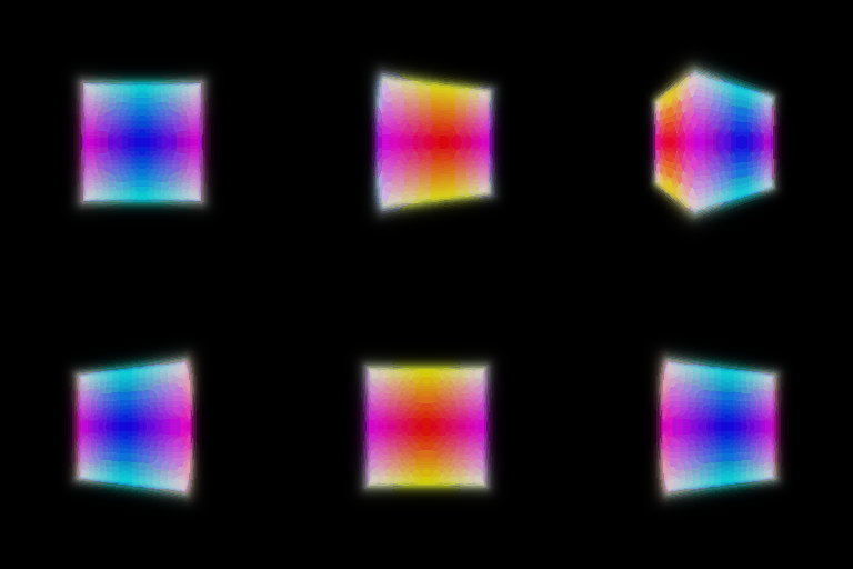
The analytic box is rendered at 256 × 256 with 64 samples per ray, near bound 0, and far bound 5.

2. Optimizing a Basic Implicit Volume
I randomly sample image pixels and minimize mean squared error between rendered RGB values and the corresponding target colors. Adam optimizes the box center and side lengths through the differentiable renderer.
Training uses four posed images, 1,000 epochs, learning rate 0.0005, and 4,096 rays per step.
| Parameter | Learned value, rounded to two decimals |
|---|---|
| Center | (0.25, 0.25, 0.00) |
| Side lengths | (2.01, 1.50, 1.50) |
The first side length is 2.005093 before rounding. Unrounded parameters.


The optimized shape is wider and offset relative to its initialization. Across the four target images, the saved final PNGs have mean RGB MSE 2.76 × 10⁻⁶, including quantization.
3. Optimizing a Neural Radiance Field
The position-only NeRF uses a six-layer position MLP with width 128 and a skip connection at layer index 3. Six harmonic frequency bands encode each 3D point into 39 channels. Density uses a ReLU output, while the color head (hidden width 64) uses sigmoid to keep RGB in [0, 1].
| Setting | Value |
|---|---|
| Dataset / image size | LEGO / 128 × 128 |
| Training | 250 epochs, Adam |
| Initial learning rate | 0.0005 |
| Ray sampling | 1,024 rays/step, 128 points/ray, depths 2–6 |
| LR schedule | Decay by a factor of 0.8 per 50 epochs |
| Validation PSNR | 24.5527 dB |
| Validation SSIM | 0.8936 |

The bulldozer, wheels, articulated arm, and platform are recognizable around the orbit. Thin details and high-frequency textures remain soft at this resolution. Full configuration.
4. NeRF Extensions
4.1 View dependence (selected extension)
Density depends only on position. The color branch additionally receives harmonic embeddings of the normalized viewing direction (two frequency bands). This allows color at a fixed location to vary with viewpoint, helping represent reflections and highlights.
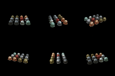
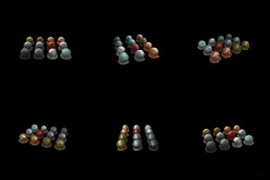
Both materials runs use 250 epochs, 128 × 128 images, initial learning rate 0.0001, 1,024 rays per step, and 128 samples per ray between depths 1 and 7.
| Materials model | Validation PSNR | Validation SSIM |
|---|---|---|
| Position only | 23.3615 dB | 0.8589 |
| View dependent | 24.3253 dB | 0.8749 |
| Change | +0.9638 dB | +0.0161 |
Trade-off: direction conditioning can model specular appearance instead of averaging it across views, but extra capacity can also memorize training-ray appearances. The compact direction branch and direction-independent geometry limit this risk. The validation improvement supports this design on the materials split; it does not establish that stronger view dependence always generalizes better.
Baseline configuration · View-dependent configuration.
4.3 VolSDF (additional experiment)
A neural surface predicts signed distance and per-point color. I convert signed distance to density with a Laplace CDF and add an Eikonal loss to encourage unit-magnitude SDF gradients. The distance network learns a residual around an initial sphere.
σ(s) = α Ψβ(−s)
L_eikonal = mean[(‖∇s‖₂ − 1)²]

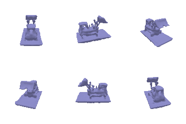
This run uses α = 10, β = 0.05, Eikonal weight 0.02, and 250 epochs. It reaches 20.6421 dB PSNR / 0.7507 SSIM. Geometry is recognizable, but the color result has blur and ghosting. Only this configuration was evaluated; no hyperparameter sweep is claimed. Configuration.
Meaning of α and β: α scales the density and therefore the strength of absorption. β controls the width of the transition from outside to inside. At the zero-level surface, density is α/2.
1. How do high and low β bias the SDF? A high β spreads density into a broad band around the surface. The network can shift the zero-level surface to compensate for opacity outside it, so the rendered and extracted boundaries need not agree closely. A low β ties opacity more closely to the zero level, favoring a sharp boundary but increasing sensitivity to sampling.
2. Which is easier to train? A moderately high β is generally easier early in training because useful density gradients reach points farther from the current surface. With very low β, uniform samples can miss the narrow transition. Extremely high β can still leave geometry poorly constrained.
3. Which is more likely to recover an accurate surface? A low β can better align the visible boundary with the zero-level surface, provided sampling resolves the narrow transition and optimization converges. Starting smoother and reducing β later is a useful future experiment, but that schedule was not evaluated here.
5. 3D Gaussian Rasterization
I construct 3D covariance matrices from rotation and squared scale, project them with a perspective Jacobian, and add 0.3 to the projected covariance diagonal for a minimum pixel footprint. Gaussian means are projected into screen coordinates. Gaussians behind the camera are filtered out, and the remaining ones are sorted front to back.
For each pixel, the Gaussian falloff times opacity gives alpha. An exclusive product of transparency gives transmittance. Color, depth, and silhouette use the resulting compositing weights. Transmittance is carried across Gaussian mini-batches.
αᵢ(x) = oᵢ exp[−½(x−μᵢ)ᵀ Σᵢ⁻¹ (x−μᵢ)]
Tᵢ(x) = Πⱼ<ᵢ [1−αⱼ(x)]
Color(x) = Σᵢ Tᵢ(x) αᵢ(x) cᵢ
All 4/4 supplied Gaussian unit tests pass.

The chair is recognizable, with streaking around elongated footprints at oblique angles. A separate post-run camera-Jacobian check identified a covariance-convention inconsistency despite the reference tests passing. These figures show the current run and have not been regenerated under a revised convention.
6. Training 3D Gaussian Representations
The toy truck uses 10,000 isotropic Gaussians initialized from the provided point cloud. Means, log-scales, opacity logits, and colors are optimized with Adam and RGB L1 loss. Quaternions are fixed in isotropic mode.
| Optimized parameter | Learning rate |
|---|---|
| Means | 0.00016 |
| Log-scales | 0.005 |
| Colors | 0.01 |
| Opacity logits | 0.01 |
| Quaternions | Not optimized (isotropic) |
Training uses 1,000 iterations, 256 Gaussians per splat, and seed 1. Held-out metrics are 24.9622 dB PSNR and 0.8590 SSIM, evaluated on five test views. Metrics and settings.
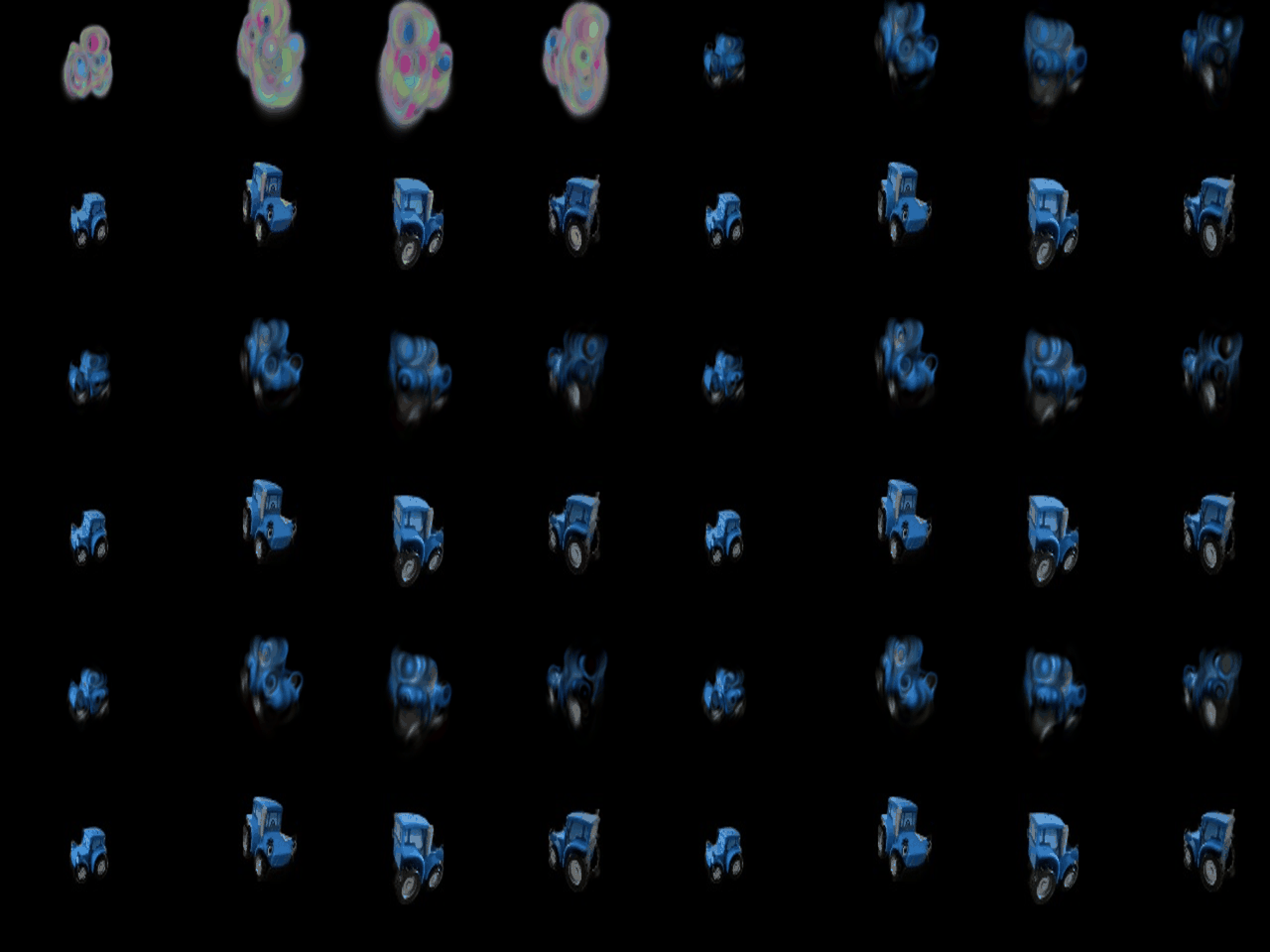

The model captures broad blue appearance but does not recover sharp cabin and wheel details. The large black background helps whole-image scores; a separate object-crop diagnostic gives about 18.09 dB PSNR. The relatively large initial splats are a plausible contributor to blur. Smaller initialization followed by retraining would be an appropriate next comparison.
7. Gaussian Extensions
7.1 Spherical harmonics (selected extension)
I evaluate real spherical harmonics through degree three, using 16 coefficients per RGB channel and the normalized camera-to-Gaussian direction. The pretrained coefficients are loaded from the PLY; new SH coefficients are not trained.

The DC-only GIF is in Section 5. The comparisons below use the exact same saved camera/frame for both methods. Depth and silhouette are unchanged across the two rendering modes.


7.2 Training on a harder scene (additional experiment)
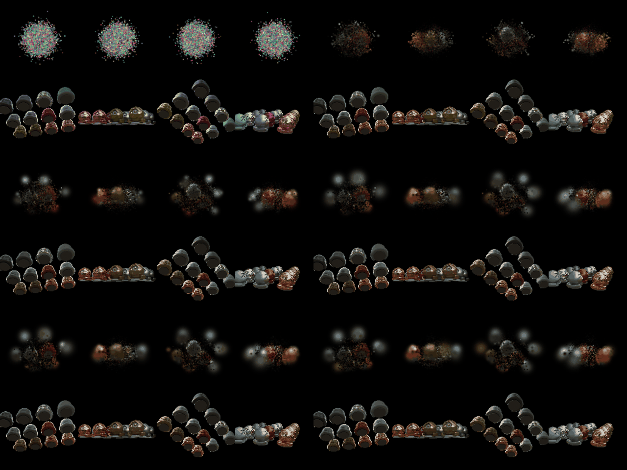
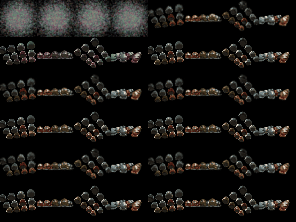
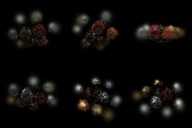
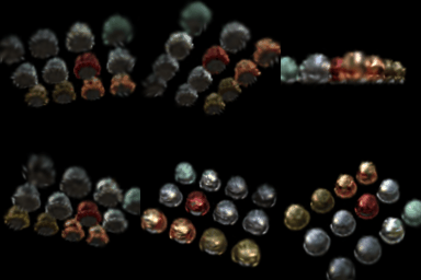
The materials baseline reuses the truck’s isotropic representation, learning rates, and L1 loss, with random means instead of point-cloud initialization. The modified method changes initialization, opacity, Gaussian shape, loss, schedule, and training duration.
| Method | Iterations | Validation PSNR | Validation SSIM |
|---|---|---|---|
| Isotropic baseline | 1,000 | 17.9657 dB | 0.6426 |
| Modified anisotropic method | 5,000 | 22.9757 dB | 0.8434 |
| Change | Baseline | Modified method |
|---|---|---|
| Gaussian shape | Isotropic | Anisotropic |
| Mean initialization | Normal, standard deviation 0.2 | Initial means × 3 (standard deviation 0.6) |
| Opacity logit | 8 (nearly opaque) | −2 (opacity ≈ 0.119) |
| Scale initialization | Random, roughly below 0.01 | Log-scale −3.5 (scale ≈ 0.0302) |
| Loss | L1 | 0.8 L1 + 0.2 (1 − SSIM) |
| Schedule | Constant learning rates | Exponential decay to approximately 10% |
| Iterations | 1,000 | 5,000 |
Initial rates match Section 6, with quaternion learning rate 0.001 added for the anisotropic run. No adaptive densification is used. Lower initial opacity allows several Gaussians to contribute, broader initialization improves coverage, and anisotropic footprints add flexibility. The combined approach improves PSNR by 5.0100 dB and SSIM by 0.2007; objects become clearer, but edges remain soft.
This is not an isolated ablation: the modified model also trains five times longer. The full gain cannot be attributed to anisotropy alone. The anisotropic result shares the covariance-convention limitation described in Section 5.
Baseline metrics and settings · Modified metrics and settings.
Summary of Measurements
| Experiment | Training | PSNR (dB) | SSIM |
|---|---|---|---|
| LEGO NeRF | 250 epochs | 24.5527 | 0.8936 |
| Materials NeRF, position only | 250 epochs | 23.3615 | 0.8589 |
| Materials NeRF, view dependent | 250 epochs | 24.3253 | 0.8749 |
| LEGO VolSDF | 250 epochs | 20.6421 | 0.7507 |
| Truck Gaussians | 1,000 iterations | 24.9622 | 0.8590 |
| Materials Gaussians, baseline | 1,000 iterations | 17.9657 | 0.6426 |
| Materials Gaussians, modified | 5,000 iterations | 22.9757 | 0.8434 |
Download measurements as CSV. Runs use seed 1. NeRF/materials images are 128 × 128; truck images are 160 × 90. Progress GIFs are resized for the webpage (640 × 320, or 512 × 256 for the modified materials run); all saved snapshots are retained. Recorded metrics are unchanged.
References
Mildenhall et al., NeRF: Representing Scenes as Neural Radiance Fields for View Synthesis (2020).
Yariv et al., Volume Rendering of Neural Implicit Surfaces (2021).
Kerbl et al., 3D Gaussian Splatting for Real-Time Radiance Field Rendering (2023).