1. Practicing with Cameras
1.1 360-degree Cow Render
I generated a complete turntable animation by varying the
camera azimuth from 0 to 360 degrees while keeping the camera
distance and elevation fixed. For every frame, PyTorch3D's
look_at_view_transform function was used to
construct the corresponding camera rotation and translation.

1.2 Dolly Zoom
The dolly zoom simultaneously changes the camera's field of view and its distance from the subject. To keep the cow at an approximately constant projected size, I maintained the following relationship:
Thus, increasing the field of view moves the camera closer, while decreasing it moves the camera farther away. The cow remains roughly the same size, but the perspective and visible plane geometry change.

2. Practicing with Meshes
2.1 Tetrahedron
A tetrahedron consists of 4 vertices and 4 triangular faces. I manually specified its vertex coordinates and constructed each face using three vertex indices.

2.2 Cube
A cube consists of 8 vertices. Each of its six square sides was divided into two triangles, producing 12 triangular faces.

3. Retexturing a Mesh
I selected blue-purple
[0.15, 0.10, 0.95] as
color1 and orange-red
[1.00, 0.20, 0.05] as
color2.
For every vertex, I normalized its z-coordinate:
The resulting value was used to linearly interpolate between the two colors:
This produces a smooth color transition along the front-to-back direction of the cow.

4. Camera Transformations
The transformed camera extrinsics were computed according to:

T_relative = [0, 0, 0].

T_relative = [-3, 0, 3] to keep the cow
centered in front of the camera.

R_relative = I and
T_relative = [0, 0, 3] move the camera farther
from the cow, making it appear smaller.

R_relative = I and
T_relative = [0.2, 0, -0.5] move the camera
closer while adding a horizontal displacement.
5. Rendering Generic 3D Representations
5.1 RGB-D Point Clouds
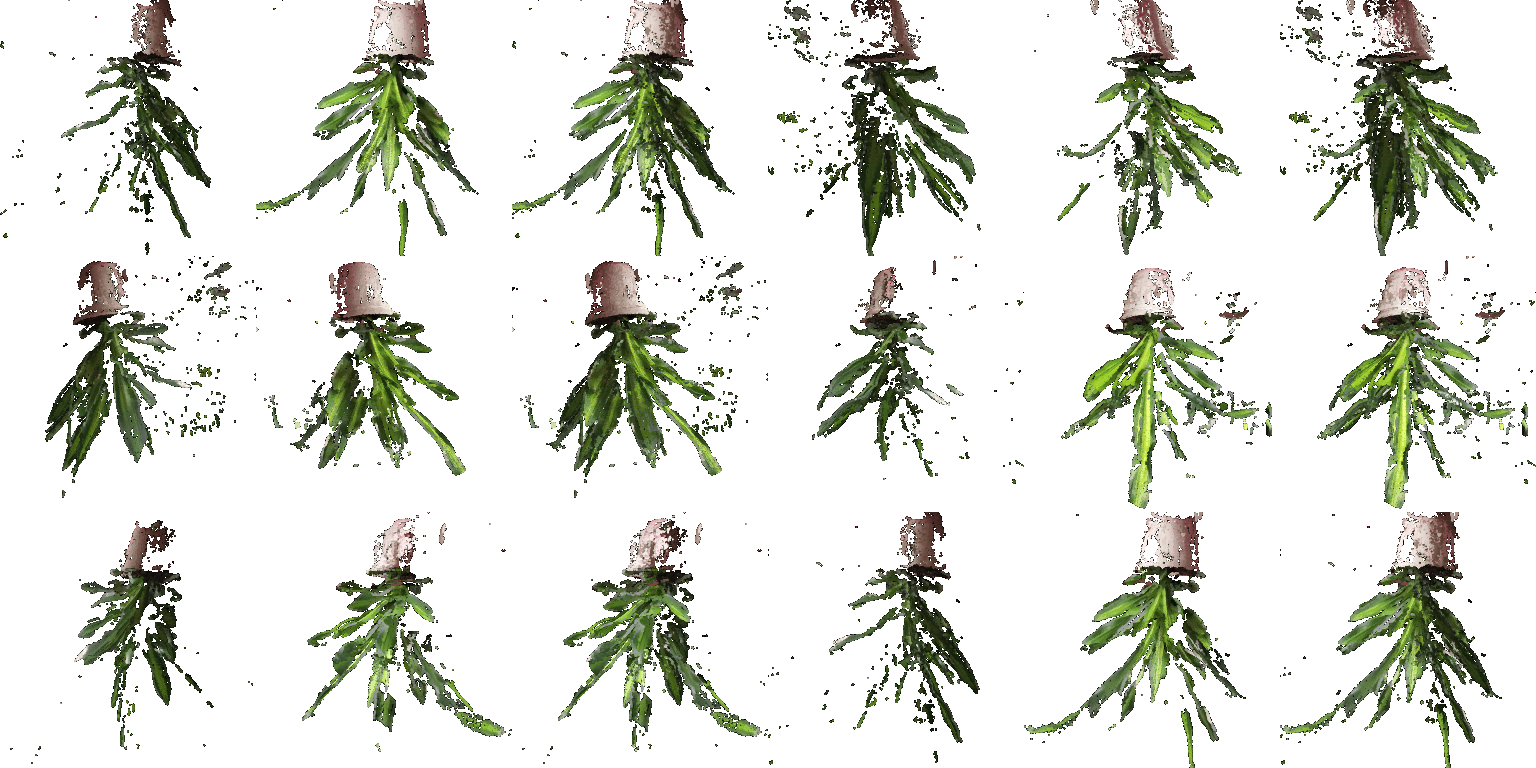
I used the supplied camera intrinsics, extrinsics, mask, and depth image to unproject every valid RGB-D pixel into a colored 3D point. I constructed separate point clouds from the two observations and created a third point cloud by concatenating their points and color features.
From left to right, the animation shows the first observation, the second observation, and their union. Each individual observation contains missing or occluded surfaces, while the union combines complementary information from both viewpoints.
5.2 Parametric Functions
Parametric Torus
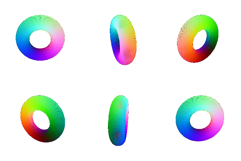
I sampled two parameters, u and v,
over the interval from 0 to 2π and evaluated:
y = (R + r cos(v)) sin(u)
z = r sin(v)
Here, R is the major radius and r is
the minor radius. The points were assigned colors derived from
their parameter values.
Custom Parametric Object: Möbius Strip
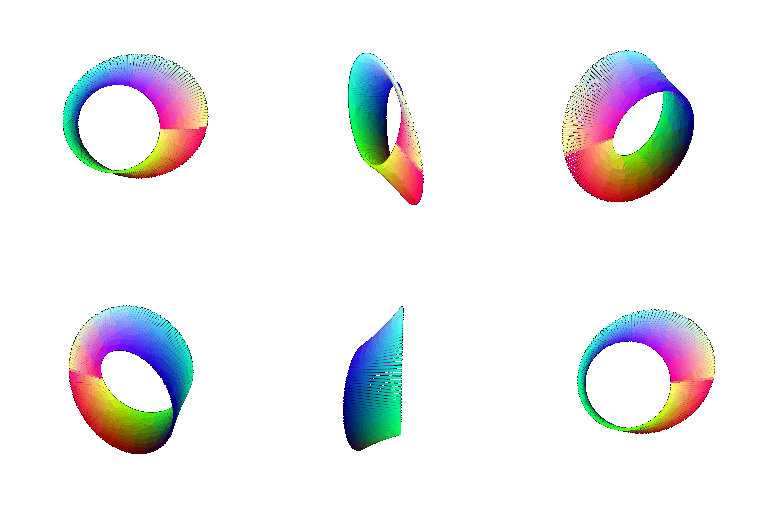
For my custom parametric object, I generated a Möbius strip, which is a one-sided, non-orientable surface. I used:
y = (1 + v cos(u/2)) sin(u)
z = v sin(u/2)
Sampling these parameters reveals the strip's characteristic half twist.
5.3 Implicit Surfaces
Implicit Torus
I defined the torus as the zero level set of:
I evaluated this function over a three-dimensional voxel grid
and applied marching cubes to extract a triangle mesh from
F(x,y,z) = 0.

Custom Implicit Object: Heart
For my custom implicit object, I evaluated a heart-shaped implicit function on a voxel grid. I then used marching cubes to extract and render its zero level-set mesh.

Mesh versus Point-Cloud Rendering
Point clouds directly represent sampled surface observations and are straightforward to construct from data such as RGB-D images. They do not require explicit surface connectivity. However, their rendering quality depends strongly on sampling density and point radius. Sparse point clouds produce visible holes, while dense point clouds require more points and memory.
Meshes explicitly represent connectivity through vertices and faces. This allows continuous surfaces, reliable surface normals, and smoother lighting. A mesh can often describe a smooth surface more efficiently than a dense point cloud. However, extracting a mesh from an implicit representation requires discretizing 3D space and running an algorithm such as marching cubes. Increasing voxel resolution improves detail, but its memory and computation grow cubically with resolution.
6. Extra Credit: Procedural Solar System
For my creative submission, I constructed a procedural miniature solar system. The scene contains several independently generated icosphere meshes with different positions, scales, and vertex colors. It includes a central sun, several planets, a moon, and a Saturn-like planet.
I generated Saturn's ring as a procedural torus triangle mesh. To combine the objects, I concatenated their vertex arrays and offset each object's face indices by the number of vertices already inserted. This produced one renderable mesh while preserving each component's geometry and colors.

7. Extra Credit: Sampling Points on Meshes
I implemented uniform surface sampling rather than simply treating the original mesh vertices as a point cloud. First, I calculated the area of every triangular face:
I selected each face with probability proportional to its area:
Area-weighted selection prevents meshes containing differently sized triangles from overrepresenting small faces and underrepresenting large faces.
After selecting a face, I sampled
r1, r2 ~ Uniform(0,1) and used the following
barycentric construction:
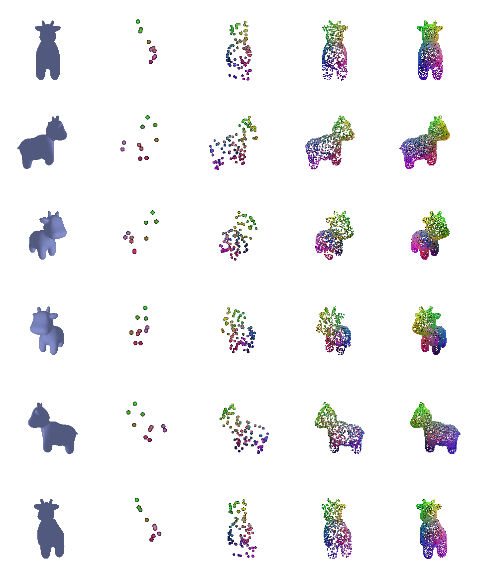
The square-root correction is required for uniform sampling over the triangle's area. With 10 points, the geometry is barely recognizable. At 100 points, its rough structure appears. At 1,000 points, the cow is clear, and at 10,000 points, the point cloud closely approximates the original continuous surface.
The panels below show the original mesh followed by point clouds containing 10, 100, 1,000, and 10,000 sampled points.