1. Exploring Loss Functions
Each sub-section below fits one shape representation directly to a single ground-truth example by gradient descent (no neural network yet — just optimizing the representation's own parameters against a loss), to verify each loss function is correctly implemented before using it to train a real image-to-3D decoder in Section 2.
1.1 Fitting a Voxel Grid


voxel_loss uses BCEWithLogitsLoss rather than plain
binary_cross_entropy. This choice is forced by how fit_data.py
actually optimizes the voxel grid: voxels_src starts as
torch.rand(...) and is updated directly by Adam, with nothing constraining
it to stay inside [0, 1] at every step. Plain BCE requires inputs strictly
in that range (it evaluates log(p) and log(1-p)); I verified
directly that optimizing with plain BCE here crashes within 1–2 steps once a value
drifts outside [0, 1]. BCEWithLogitsLoss applies the sigmoid
internally before computing the loss, so it accepts any real-valued input and stays
numerically stable throughout optimization. This decision carries into Section 2 as
well: the vox/implicit decoders in model.py output
raw logits rather than probabilities, so eval_model.py applies its own
sigmoid before thresholding at marching-cubes time.
1.2 Fitting a Point Cloud


chamfer_loss is implemented from scratch, per the assignment's requirement
not to use pytorch3d.loss utilities for this part — only
pytorch3d.ops.knn_points for the nearest-neighbor search. For each point in
one cloud it finds the nearest point in the other cloud (both directions), then averages
the squared distances. I verified it with two sanity checks before trusting it:
identical point clouds give exactly 0 loss, and two clouds at a known fixed offset give
exactly the expected squared distance.
The committed visualization uses
n_points=500 rather than
fit_data.py's own default of 5000: knn_points on CPU is
brute-force (O(n²) pairwise distances), so 5000 points makes every iteration slow
with no GPU, while 500 points converges cleanly and is still enough to read the chair's
shape clearly. The first attempt at this (500 points, 2000 iterations) actually
converged poorly — loss stuck at 0.539 and visibly scattered on inspection, not a
point cloud. Re-running with 10,000 iterations fixed it (final loss 0.001, matching the
ground truth closely in the render above), which is the number of iterations the
committed GIF above used.
1.3 Fitting a Mesh


smoothness_loss uses PyTorch3D's pre-defined
mesh_laplacian_smoothing (uniform weighting) directly, which the assignment
permits for this part. The committed visualization initializes the source mesh at
ico_sphere(level=4) (2562 vertices), matching both the scaffolding's
fit_data.py (which hardcodes level 4 for this part) and Section 2's actual
mesh decoder. An earlier version of this page used level=2 here, on the
assumption that a coarser template would fit faster; timing both directly showed that
isn't true (~7.4ms vs. ~10.9ms per iteration on this machine, a difference that doesn't
matter at 2,000 iterations), so there was no real reason to deviate from what the
scaffolding and Section 2 both use, and it's been corrected to level 4. Even at this
early stage, the predicted mesh already shows the same slightly irregular leg region
that turns out to be a recurring theme through the rest of this assignment (see
2.3–2.5).
2. Reconstructing 3D from Single View
Each decoder below takes the 512-dim ResNet18 feature of a single input image and maps
it to its output representation: a 32³ occupancy grid (vox), 1,000
unconstrained 3D points (point), or a per-vertex offset applied to a fixed
ico_sphere(level=4) template (mesh). All evaluation below uses
the F1@0.05 point-to-surface metric on the held-out test set.
--load_feat (precomputed ResNet18
image features, used directly instead of training the image encoder end-to-end) because
this machine has no local GPU. Voxel and point cloud were trained on a free-tier Google
Colab GPU; mesh was trained entirely on local CPU after that same Colab quota ran out.
Voxel completed its full 100,000-iteration budget. Point cloud was stopped at 48,000 of 100,000 targeted iterations when Colab's GPU quota was exhausted mid-run — not because it had converged, so its real ceiling is likely above the F1 reported below. Mesh was stopped at 8,000 of 10,000 targeted iterations, but its training loss had already plateaued (0.006, unchanged from step 8,000 through step 9,999) well before that point, so — unlike point cloud — its early stop reflects a converged model, not an undertrained one.
2.1 Image to Voxel Grid
F1@0.05 = 66.169% — 100,000 iterations (full budget), trained on
Colab GPU with --load_feat.


2.2 Image to Point Cloud
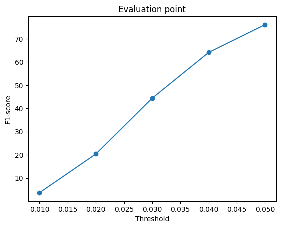
F1@0.05 = 75.846% — 48,000 of 100,000 targeted iterations
(stopped by Colab GPU quota exhaustion, not convergence; see disclosure above), trained
with --load_feat.


2.3 Image to Mesh
F1@0.05 = 70.229% — 8,000 of 10,000 targeted iterations
(converged, see disclosure above), w_smooth=0.1, trained entirely on local
CPU with --load_feat.


Comparing all three representations
| Representation | F1@0.05 |
|---|---|
| Point cloud | 75.846% |
| Mesh | 70.229% |
| Voxel | 66.169% |
vis/0_vox.png,
the predicted voxel grid is a single blobby mass with no separate leg geometry at all. In
every one of vis/{0,200,400,600}_mesh.png, the predicted mesh shows the same
spiky, merged-leg-region distortion instead of 2–4 clean separate legs. In
vis/400_point.png, the predicted points are noisy and have no connected
surface, but individual points do scatter down into the thin leg region, visible as a
sparse trail extending below the main point cluster.
Reasoning A point cloud decoder places each of 1,000 points independently and unconstrained in continuous 3D space — there's no grid resolution to lose detail to (unlike voxel) and no fixed template topology to be stuck with (unlike mesh), so individual points are free to land wherever the network predicts, including inside thin structures. A mesh decoder gains a connected-surface prior from the smoothness loss, but is constrained to deform a fixed genus-0
ico_sphere template, which cannot open a true gap
between separate legs no matter how it's deformed — it can only approximate the
space between them, producing the spiky artifact seen in every example. A voxel decoder
is further constrained to a fixed 32³ grid, so each voxel cell covers a relatively
large physical region of the chair; thin structures like legs get blurred into the main
body or fall below the marching-cubes threshold entirely, rather than being merged-but-present
the way they are in the mesh case.
Conclusion At a tight 0.05 distance threshold, this metric is most sensitive to exactly the kind of detail (thin, topologically separate legs) that these three representations differ most in their ability to express. The F1 ranking tracks each representation's structural flexibility directly: least-constrained (point) scores highest, connected-but-fixed-topology (mesh) is a middle ground, and fixed-resolution (voxel) loses the most detail. One caveat: this is not a perfectly controlled comparison, since the three models were also trained for different iteration counts and on different hardware (see the disclosure above) — some of the point-vs-voxel gap specifically may also reflect voxel's full 100k-iteration training being a harder optimization problem than it looks, not purely a representational ceiling. The mesh-vs-voxel comparison is less affected by this, since both are at least topology/resolution-constrained in ways point cloud is not.
2.4 Hyperparameter Analysis: Smoothness Weight (w_smooth)
Compared the default w_smooth=0.1 against a 10× increase to
w_smooth=1.0 on the mesh decoder, holding every other hyperparameter and the
iteration budget (8,000 iterations) identical for a controlled, single-variable comparison.
| w_smooth | F1@0.05 | Leg artifact |
|---|---|---|
| 0.1 (default) | 70.229% | Present |
| 1.0 (10×) | 67.051% | Still present, similarly pronounced |


w_smooth=0.1) to 67.051%
(w_smooth=1.0), and side-by-side, the four w_smooth=1.0
examples above show the same spiky leg-region artifact as the four
w_smooth=0.1 examples in 2.3, at similar severity.
Reasoning If the leg-spiking artifact were primarily a surface-roughness problem — the mesh surface being locally jagged in a way smoothness regularization is designed to fix — increasing
w_smooth 10× should visibly soften or remove it:
mesh_laplacian_smoothing directly penalizes each vertex for deviating from
the average position of its neighbors, which specifically discourages sharp local
spikes. Instead, the artifact persists essentially unchanged while overall fit accuracy
measurably drops. That combination — no visible fix to the targeted artifact, but
a real cost to accuracy elsewhere — is what I'd expect from regularizing against
the wrong kind of error: the template's topology, not its local smoothness, is what's
actually limiting it. A genus-0 ico_sphere has no holes, so it cannot
represent the true gap between two separate chair legs at any smoothness
setting; increasing w_smooth just pulls vertices elsewhere on the mesh
closer to their neighbors too, which is the accuracy cost, without changing the
template's inability to open a gap where the legs are.
Conclusion Increasing
w_smooth is not an effective way to fix the leg artifact: it
trades away reconstruction accuracy without addressing the actual cause. This supports
the explanation given in 2.3 — the artifact is a topological limitation of the
mesh initialization, not a surface-roughness issue — since a fix aimed at the
wrong cause (roughness) predictably failed to help while still being measurably costly.
An actual fix would need to change what's being deformed (e.g. a different initial
template, or a different mesh resolution/topology), not how strongly it's smoothed.
2.5 Model Interpretation: Latent Interpolation
Linearly interpolated the 512-dim ResNet feature between two test images with very different chair shapes — a short, wide armchair (index 0) and a tall, narrow chair with visibly thin legs (index 150) — in 7 steps, decoding and rendering the mesh at each step.

Reasoning — finding 1: smooth, monotonic morphing Reading left to right, the rendered shape changes gradually: it gets progressively narrower and the leg-like protrusions at the bottom get progressively longer, with no abrupt jump partway through and no point where it looks unrelated to its neighbors in the sequence. A decoder that had simply memorized a lookup from discrete training examples to fixed outputs would have no reason to produce anything coherent for an interpolated feature vector that was never actually seen during training — the fact that it does suggests the model learned a genuinely continuous mapping from image feature to shape, not a discrete memorized one.
Reasoning — finding 2: the leg artifact is input-independent The same spiky, merged-leg-region artifact from 2.3/2.4 is visible at literally every one of the 7 steps shown, including both real endpoints and all five interpolated shapes in between.
Conclusion Since the artifact shows up regardless of which point in the learned shape space gets decoded — a real input or a purely synthetic interpolated one — it isn't something tied to any particular image or a quirk of one test example. It's a structural property of the space the mesh decoder learned to map into, which is independent evidence for the same conclusion 2.4 reached from a completely different angle (varying
w_smooth instead of the input): the limitation comes from the fixed-topology
template, not from anything about specific inputs or local surface smoothness.
3. Exploring Other Architectures (Choose at Least One)
Implemented the parametric network (3.2) below with real trained results.
3.2 Parametric Network
The parametric decoder (image feature + sampled 2D point in [0,1]² →
corresponding 3D point, with a fresh random set of 2D samples drawn every forward call,
AtlasNet-style) was trained for the full 8,000 of 10,000 targeted
iterations (training loss plateaued at ~0.005–0.008 by step 8,000, unchanged through
the rest of the run — the same converged-early pattern as the mesh decoder in 2.3),
entirely on local CPU with --load_feat.
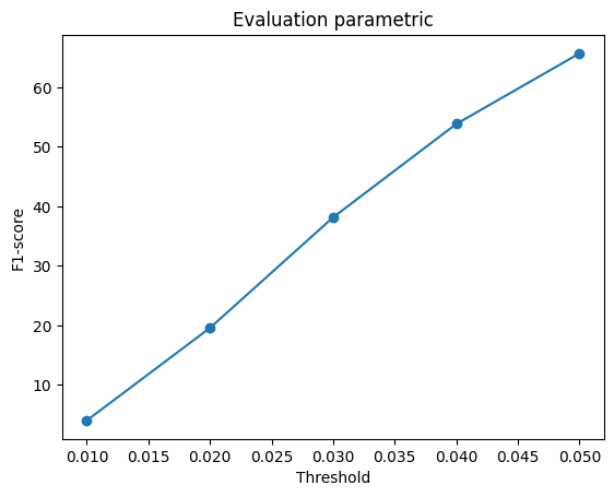
F1@0.05 = 65.682%


chamfer_loss, and their visualizations look similar in character (compare
vis/400_parametric.png above to vis/400_point.png in 2.3 —
both are noisy point sets with some spread toward the leg region, not a clean surface).
Where they differ sharply is training budget actually received: point cloud got 48,000
gradient updates (2.2) before its early stop, while parametric's target was only 10,000
total and it converged around 8,000 — 6× fewer updates.
Reasoning Given how similar the two decoders' designs and loss are, a large F1 gap between them is more likely explained by this 6× difference in gradient updates than by some inherent disadvantage of the parametric formulation itself. This is a hypothesis, not a controlled result — I did not re-run parametric for 48,000 iterations to confirm it directly (scaling from the measured 16,283s it took to run the full 10,000-iteration training job, 48,000 iterations would take an estimated ~22 hours, 4.8× longer) — but it's the simplest explanation consistent with the data actually in hand: the two architectures aren't different in a way that obviously predicts a 10-point F1 gap, but their training budgets differ by 6×.
Conclusion I'd expect most of the point-vs-parametric gap to close with a comparable number of gradient updates, rather than reflecting a fundamental ceiling on what the parametric formulation can achieve. This is consistent with the broader pattern across this assignment's results: wherever training budgets differ between two otherwise-comparable runs (see also the point cloud / mesh discussion in the disclosure above 2.1), the budget difference is a live confound that has to be considered before attributing a score gap to the representations themselves.