Assignment 3: Neural Volume Rendering and Gaussian Splatting
Contents
- A. Neural Volume Rendering: 1.3, 1.4, 1.5, 2, 3, 4.1, 4.2, 4.3
- B. 3D Gaussian Splatting: 5, 6, 7.1, 7.2
A. Neural Volume Rendering
1.3 Ray sampling (5 points)
| xy_grid | Rays |
|---|
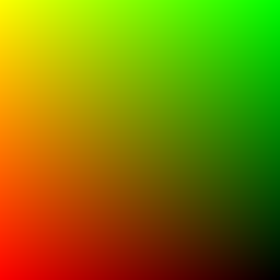 | 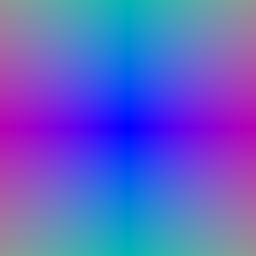 |
1.4 Point sampling (5 points)
| Point samples from first camera |
|---|
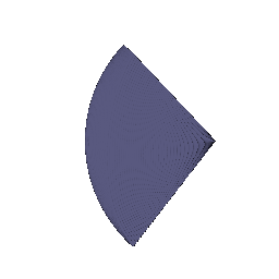 |
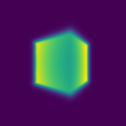
1.5 Volume rendering (20 points)
| Rendered box | Depth normalized by its maximum value. |
|---|
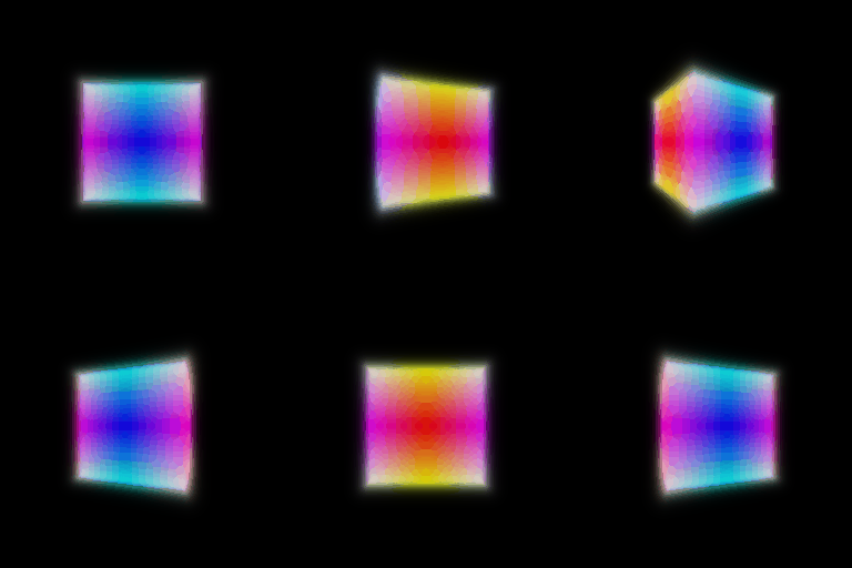 |  |
2. Optimizing a basic implicit volume (2.1 to 2.3)
After training with the MSE loss on random rays:
| Center of box | (0.25, 0.25, 0.00) |
|---|
| Side lengths of box | (2.01, 1.50, 1.50) |
|---|
| Optimized box |
|---|
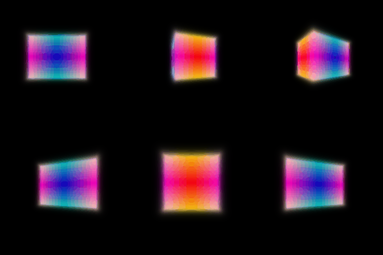 |
It looks the same as ta_images/part_2.gif.
3. Optimizing a Neural Radiance Field (20 points)
| NeRF on lego, 128x128 |
|---|
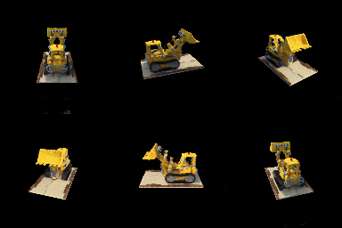 |
I kept the base settings in nerf_lego.yaml. My model reaches 24.1 dB validation PSNR. The fine detail on the tracks and the arm is a little blurry at this resolution, and there is a small floater artifact near the bulldozer in some views.
4.1 View dependence (10 points)
I embedded the viewing direction with 2 harmonic functions and concatenated it to the features after the density head, so density stays a function of position only.
| Materials, 128x128 | Train PSNR | Val PSNR |
|---|
| No view dependence | 23.44 | 23.30 |
| View dependence | 24.44 | 24.26 |
| No view dependence | View dependence |
|---|
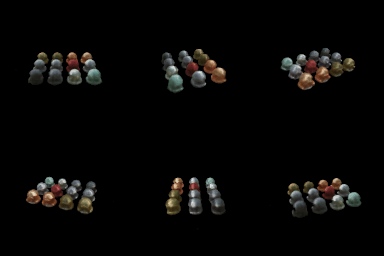 | 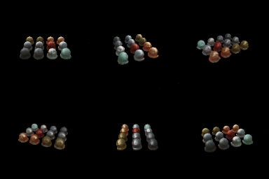 |
Adding view dependence improved my validation PSNR by about 1 dB. The spheres are made of different materials, and the shiny ones have highlights and reflections that change with the camera, which a color that depends only on position can't fit. The gap between train and val PSNR stays small (0.18 dB vs 0.14 dB), so I don't see overfitting here.
The trade-off is that the more the color can depend on direction, the more the network can explain each training image with color instead of geometry, for example by memorizing per-view effects or painting a view-specific color onto a floater. That doesn't carry over to new views. This is why I added the direction late, through a small head and with only 2 frequencies. More frequencies, an earlier direction input or fewer training views would likely raise train PSNR and lower val PSNR.
View dependence, 400x400 (nerf_materials_highres.yaml) |
|---|
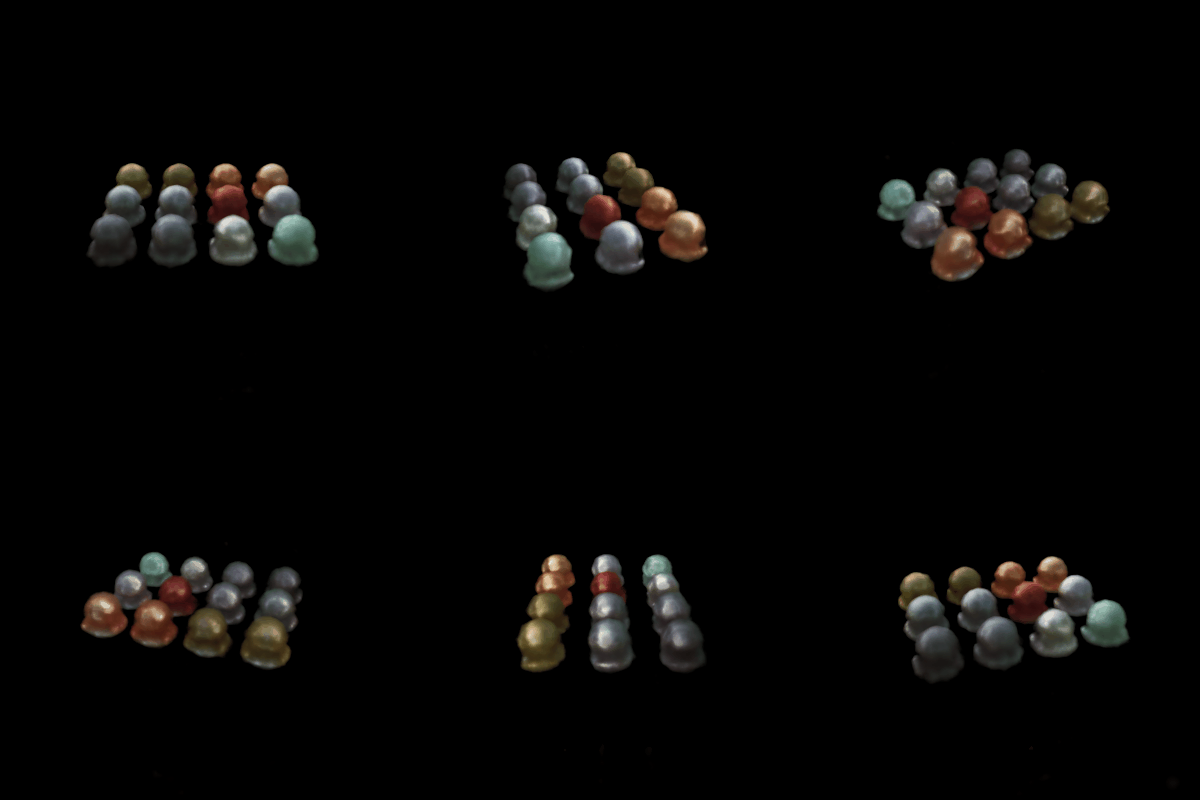 |
At 400x400 the model reaches 24.39 dB val PSNR, and the renders appear sharper.
4.2 Coarse/Fine sampling (10 points)
I used two NeRF MLPs with the same architecture that I used in Part 3. I evaluated the coarse one on 64 evenly spaced samples. Its weights give a piecewise-constant PDF along each ray, and I draw 128 more samples from it by inverse transform sampling.
I evaluated the fine network on all 192 sorted samples. The total loss is the MSE of the fine render plus the MSE of the coarse render.
| Lego, 128x128 | Network evaluations per ray | Train time | Render time | Val PSNR |
|---|
| Single network, 128 samples (Part 3) | 128 | about 11 min | 0.29 s/image | 24.13 |
| Coarse/fine, 64 + 128 samples | 64 + 192 | about 19 min | 0.45 s/image | 24.98 |
| Single network | Coarse/fine |
|---|
|  |
Adding coarse/fine sampling adds about 0.85 dB. The visual difference in the GIFs is small, but it costs twice the parameters, about 1.7x the training time and roughly 1.5x the render time.
4.3 VolSDF (10 points)
I used the position MLP from Part 3 as the distance MLP, with a linear output (no ReLU) since an SDF can be negative. The color head is a 2-layer MLP with a Sigmoid on the same features. Density is alpha * Psi_beta(-d), where Psi_beta is the CDF of a zero-mean Laplace distribution with scale beta. The loss adds the eikonal term (weight 0.02) on points sampled in the bounding box.
alpha is the density deep inside the object and essentially sets how opaque the inside is.
beta sets how wide the transition is meaning density goes from 0 outside to alpha inside over a band of a few beta around the zero level set. With a small beta the surface is sharp. With a large beta it is a soft, thicker shell.
- How does beta bias the learned SDF?
High beta biases the learned SDF by leaking density out to points well outside the surface, so rendered color would come from a thick shell around the zero level set. This pushes the SDF toward smooth and rounded shapes, and its zero level set doesn't have to sit exactly on the visible surface.
With a low beta, density is close to an indicator of the inside, so the SDF is less biased, but only points close to the zero level set affect the image.
- Easier to train with high or low beta? I think it would be easier to train with high beta. Many samples along each ray get a non-zero density and gradient, so we are still giving the SDF a signal even when its surface is far from the right place. When we have a low beta the gradient would only exist in a thin band around the current surface that I think would make optimization from a random start harder.
- More accurate surface with high or low beta?
I think you would be more likely to learn an accurate surface with low beta. The rendered color would come from the zero level set, so matching the images would pin the surface down. A high beta would just blur where the surface is.
| beta (alpha 10) | Train PSNR | Val PSNR |
|---|
| 0.02 | 22.69 | 22.47 |
| 0.05 (config default) | 22.25 | 22.08 |
| 0.1 | 21.45 | 21.32 |
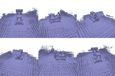
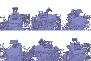
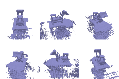
| beta 0.02 | beta 0.05 | beta 0.1 |
|---|
 |  |  |
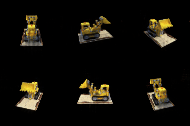 | 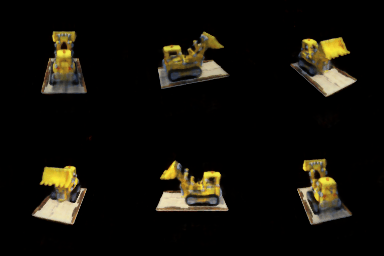 | 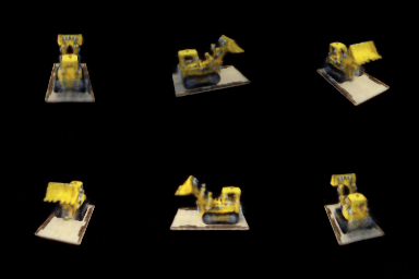 |
I varied beta and kept everything else consistent. Lower beta gives higher PSNR but every run also produces extra surfaces in empty space around the bulldozer that grow as beta gets smaller and are much reduced at beta 0.1.
These regions are black in the training images (black background), so the color loss likely doesn't penalize them.
With a small beta, gradients are confined to a thin band, so nothing removes them once they form. With a larger beta, the wider band lets the loss see and remove them.
My choice is beta 0.1 since it gives the cleanest geometry at a cost of about 0.8 dB compared with the default.
B. 3D Gaussian Splatting
5. 3D Gaussian Rasterization (35 points)
| 5.5: render, depth and mask |
|---|
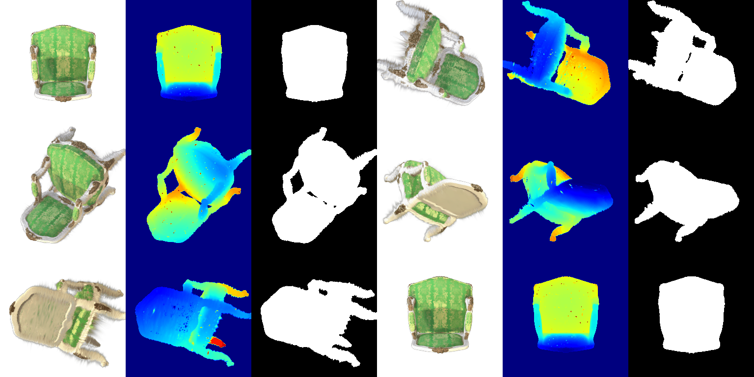 |
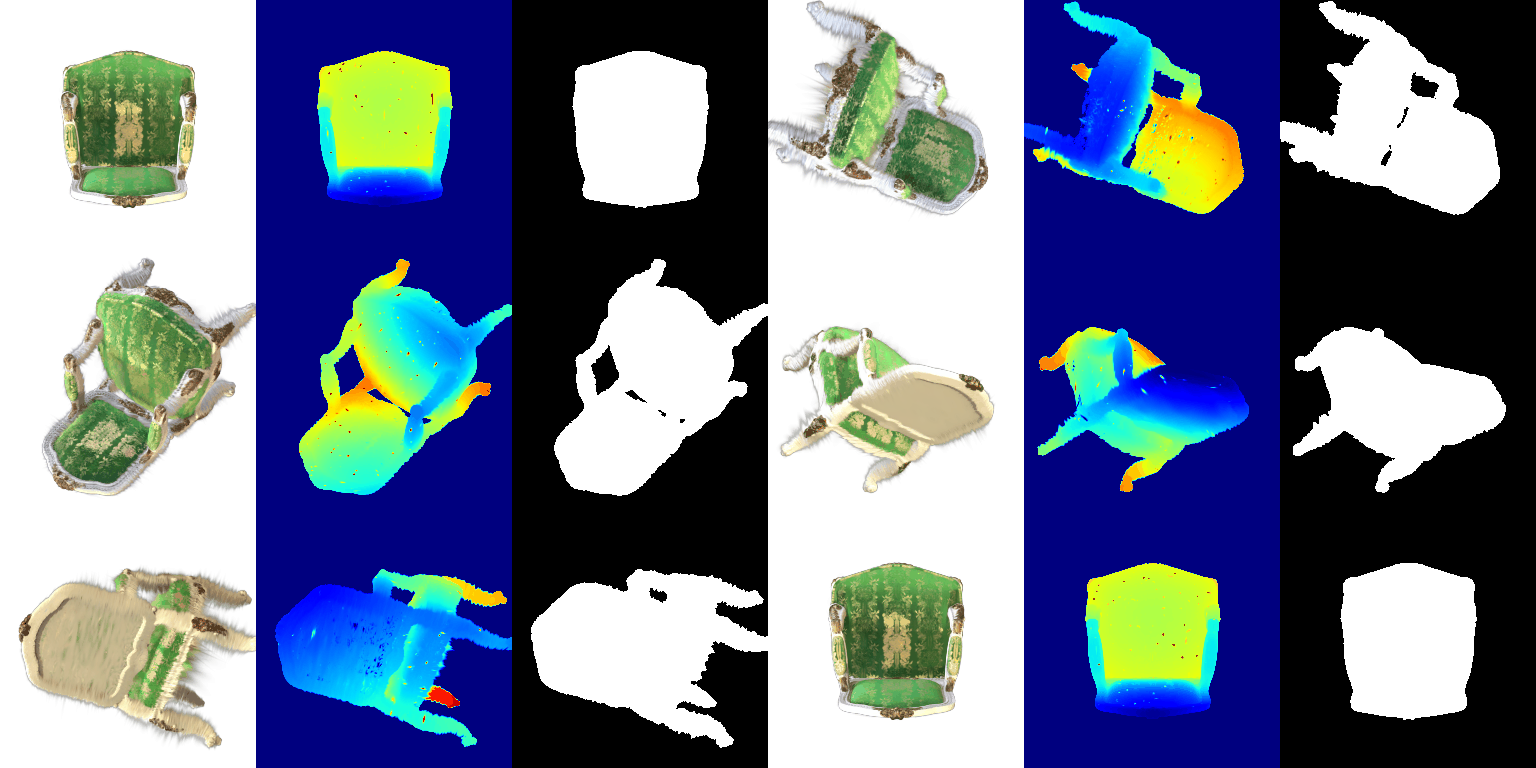
Some thin parts like the legs show streaks. This comes from the rotation W in the 2D covariance J W Sigma W^T J^T. The unit test for compute_cov_2D expects W to be camera.R, so that is what I used and the Piazza post confirmed this was fine.
Still, pytorch3d stores R for row vectors, so the actual world-to-camera rotation that acts on column vectors is R^T. Using R^T makes the streaks go away, but two unit tests then fail.
| W = R^T (left) and W = R (right) |
|---|
 |
6. Training 3D Gaussian Representations (15 points)
| Parameter | Adam Learning rate |
|---|
| Opacities (pre-activation) | 0.05 |
| Scales (pre-activation) | 0.005 |
| Colors | 0.02 |
| Means | 0.0005 |
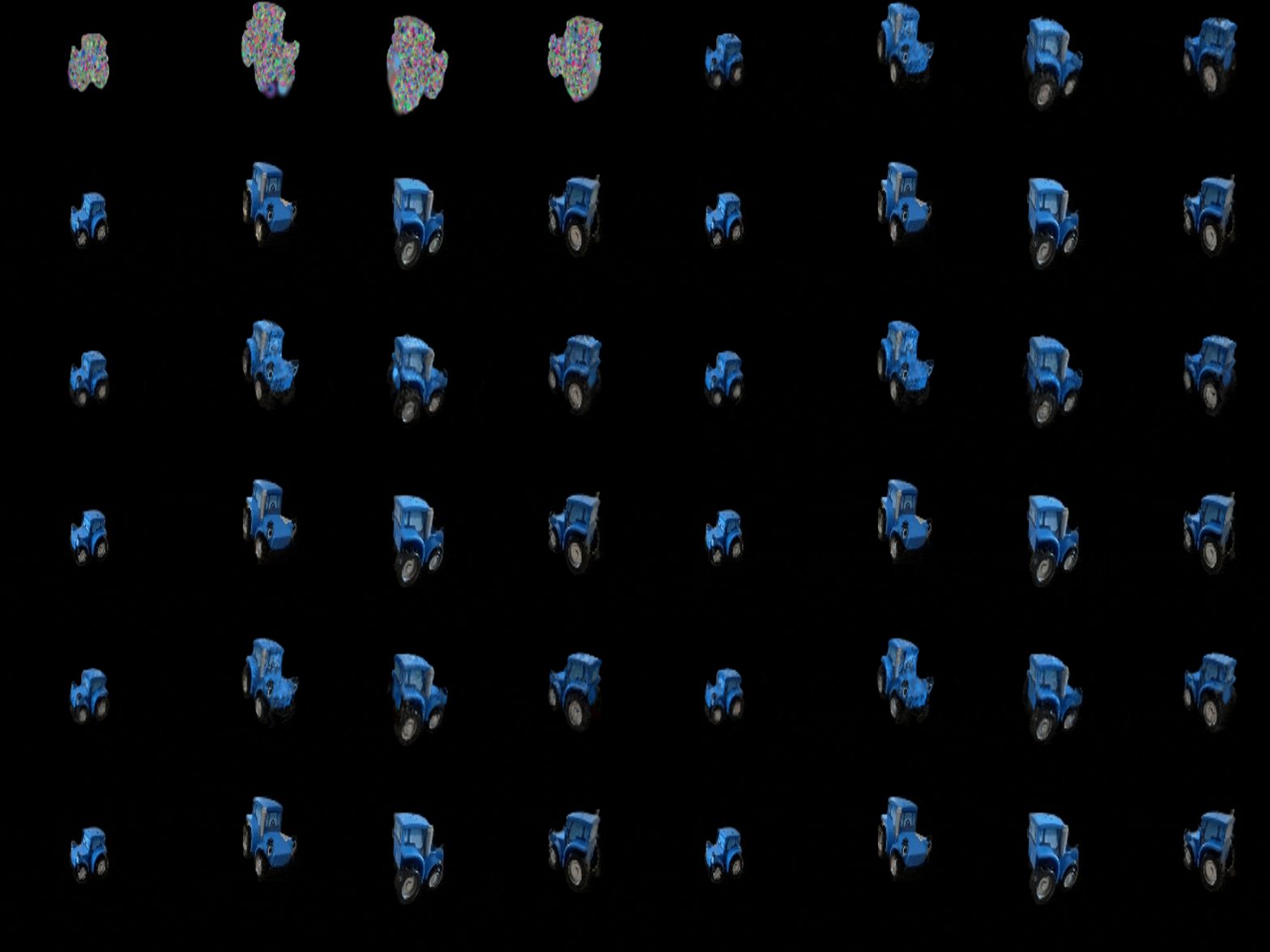
I trained for a default 1000 iterations with an L1 loss and isotropic Gaussians initialized from the given point cloud.
On the test views the model gets PSNR 29.83 and SSIM 0.942. Means get the smallest learning rate since the point cloud already puts them close to the right place, and opacity and color get the largest since they need to move a lot from their initial values. I used --gaussians_per_splat 1024 for training with gradient checkpointing for each mini-batch of Gaussians. I made the final renders GIFs on this page play at 150 ms per frame instead of the script's 100 ms and compressed the progress GIFs to keep the page size within memory constraints.
| Training progress (render@top, ground truth @bottom) |
|---|
 |
| Final renders |
|---|
 |
7. Extensions
7.1 Rendering using spherical harmonics (10 points)
| DC color only (5.5) | Spherical harmonics, degree 3 |
|---|
|  |
DC (left) and spherical harmonics (right):
| Frame 0 |
|---|
 |
On the initial frame with SH the fabric on the backrest and seat is a darker, more saturated green, and the gold pattern stands out more. The DC color is roughly the average over all viewing directions, so it washes out the sheen of the fabric.
| Frame 8 |
|---|
 |
Here again the green is darker and has more contrast with SH, and the shading on the curved seat is stronger and gives it more shape.
| Frame 24 |
|---|
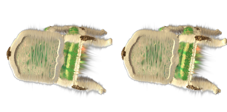 |
These two are almost identical. From here the matte underside of the seat and the wooden legs probably look about the same from every direction.
7.2 Training on a harder scene (10 points)
| Materials, val split | Iterations | PSNR | SSIM |
|---|
| Baseline (same as Q6) | 1000 | 18.58 | 0.682 |
| Improved | 3000 | 23.90 | 0.876 |
The baseline has 10k isotropic Gaussians with the default random init and follows Q6 params. The improved run uses these learning rates:
| Parameter | Adam Learning rate |
|---|
| Opacities (pre-activation) | 0.05 |
| Scales (pre-activation) | 0.005 |
| Colors | 0.02 |
| Means | 0.001, decayed exponentially to 0.00001 |
| Quaternions | 0.001 |
| Baseline training |
|---|
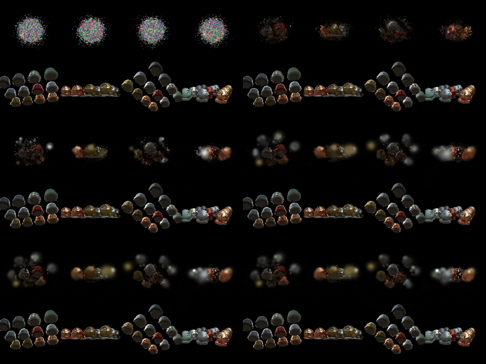 |
| Improved training |
|---|
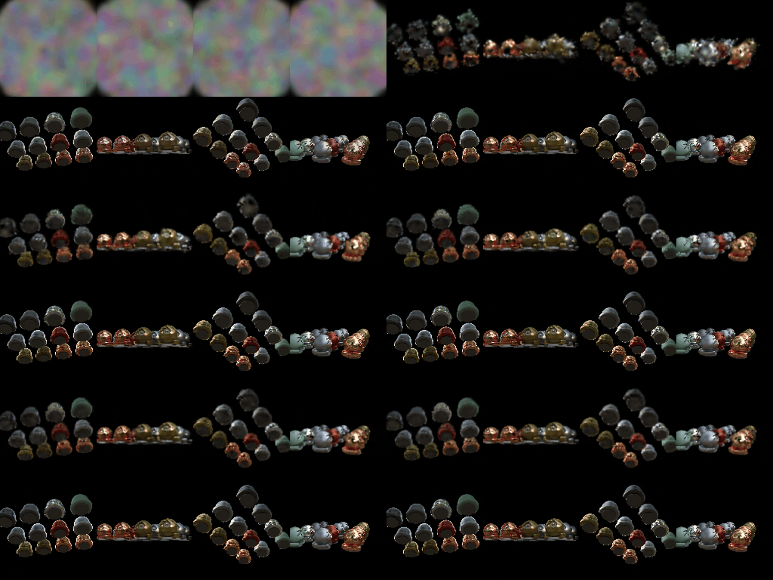 |
| Baseline final renders | Improved final renders |
|---|
 |  |
The improved run gains 5.3 dB PSNR and 0.19 SSIM. In the baseline progress the Gaussians start as a small cloud around the origin and spread out slowly but are still blurry overlapping blobs at the end.
The improved run covers every sphere within the first few hundred iterations, and by the middle of training they are separate with visible shading. The edges are still soft and the reflections blurry (which is expected for view-independent color). Compared to Q6:
- I sampled the means uniformly in a ball of r=1.5 that covers all the spheres and set each initial scale to the mean distance to its 3 nearest neighbors. I also started at opacity=0.1 like the 3DGS paper which lets Gaussians behind the front ones still get gradients.
- Quaternions are trained, so a Gaussian can stretch along a sphere's surface instead of needing several round ones.
- For the loss I used 0.8 L1 + 0.2 (1 minus SSIM) as in the 3DGS paper, with my own differentiable SSIM (with an 11x11 Gaussian window). SSIM rewards local structure that seems to help the edges of the spheres.
- I set the means learning rate to 0.001 (twice Q6) so they can travel from random positions, then decay exponentially to 1% of that so they settle at the end.
- Every 100 iterations from iteration 500 to 1800, I took the 5% of Gaussians with the largest average gradient of the mean. I cloned the small ones (largest scale 0.02 or less) and split large ones into two copies offset by a sample from the Gaussian with scales divided by 1.6. I pruned Gaussians with opacity below 0.005 which ended up removing more than the densification added and the run ended with 4,877 Gaussians, less than half of the baseline's 10k.
- I also trained longer, 3000 iterations instead of 1000. I didn't train the baseline for 3000 iterations, so part of the gap may come from that, but the baseline's L1 loss was decreasing only slowly by the end, so I expect most of the gap is due to the other changes.