16-825: Assignment 3: Volume Rendering, NeRF and 3D Gaussian Splatting
Abhikhya Tripathy (Andrew ID: abhikhyt)
Part A: neural volume rendering. Part B: 3D Gaussian splatting.
1. Differentiable Volume Rendering
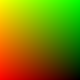
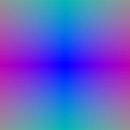
1.3 Ray sampling
Each pixel is mapped to the range [-1, 1], placed on the image plane at depth 1, and unprojected to world space. Each ray starts at the camera center and points through its pixel; the direction is normalized.
1.4 Point sampling
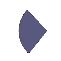
64 depths are spaced evenly between near and far. Each sample point is origin + depth × direction.
1.5 Volume rendering
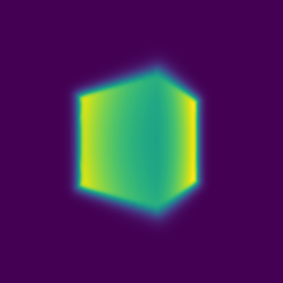
For each sample, alpha = 1 − exp(−σ·Δt). Transmittance T is the product of (1 − alpha) over all earlier samples, with T = 1 for the first one. Each sample's weight is T · alpha. Color is the weighted sum of sample colors, and depth is the weighted sum of sample depths.

2. Optimizing a Basic Implicit Volume
2.1 Each training step uses a random subset of pixels: all pixel coordinates are shuffled and the first N are kept. This saves GPU memory.
2.2 The loss is the mean squared error between rendered and ground-truth colors.
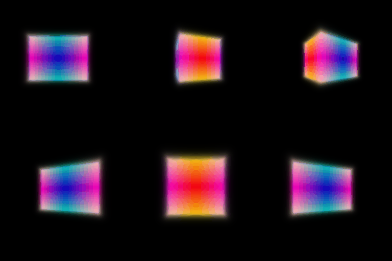
| x | y | z | |
|---|---|---|---|
| Box center | 0.25 | 0.25 | 0.00 |
| Box side lengths | 2.01 | 1.50 | 1.50 |
3. Optimizing a Neural Radiance Field
Network: the 3D position is positionally encoded with 6 frequencies, then passed through a 6-layer MLP (128 units, ReLU). The input is re-injected at layer 3 (a skip connection). Two heads follow:
- Density:
Linear → ReLU, so density is never negative. - Color:
Linear → ReLU → Linear → Sigmoid, so color stays in [0, 1].
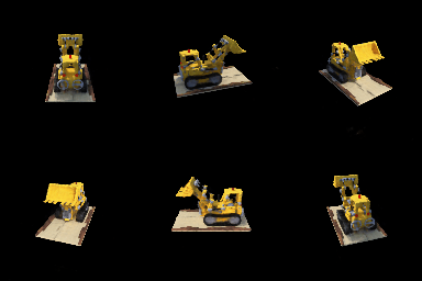
Training: MSE loss, 250 epochs on 128×128 lego images.
4. NeRF Extras (all three done)
4.1 View dependence
How: the viewing direction is encoded with 2 frequencies and added only to the color head, after the position MLP. Density still depends on position only, so the geometry cannot change with viewpoint.
To answer the trade-off questions with numbers, not just by eye, we measure PSNR (higher is better) on held-out views the model never trained on. This shows how well each model generalizes to new viewpoints.
| Materials scene | Held-out PSNR |
|---|---|
| 128×128, no view dependence | 23.43 dB |
| 128×128, with view dependence | 24.09 dB |
| 400×400, with view dependence (lr 5e-4) | 26.03 dB |

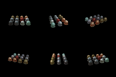

Trade-off: view dependence lets shiny materials show highlights that move with the camera. With it, held-out PSNR rose by 0.7 dB. The risk is overfitting: a network that leans too much on direction can "paint" each training view separately instead of learning one consistent 3D scene, and new views then look wrong. We limit this in three ways:
- Density never sees the direction.
- The direction uses only 2 encoding frequencies, so it can only vary smoothly.
- The direction enters late, through a small head.
Generalization improved rather than dropped, so this amount of view dependence is a good balance.
At 400×400, the default learning rate (1e-4) collapsed to an empty scene (15.38 dB). Most rays hit black background, so the ReLU density head "died" early and output zero density everywhere. A higher learning rate (5e-4) fixed it.
4.2 Coarse/fine sampling
How: two networks.
- The coarse network is evaluated at 64 evenly spaced samples. Its weights show where the surface probably is.
- We then draw 128 extra samples from those weights (inverse-CDF sampling), so samples cluster near the surface.
- The fine network renders all 192 samples.
- Both networks are trained with MSE.
| Lego | Samples / ray | Held-out PSNR | Training speed |
|---|---|---|---|
| Single NeRF (Q3) | 128 uniform | 24.51 dB | ≈ 78 it/s |
| Coarse + fine | 64 + 128 | 24.92 dB | ≈ 44 it/s |

Trade-off: samples near the surface matter most, and the fine pass puts them there. Quality goes up (+0.4 dB, sharper edges), but each step runs two networks on more points, so training is about 1.8× slower. The two runs used different GPU nodes, so the speed ratio is approximate.
4.3 VolSDF
How:
- Distance network: a 6-layer MLP (128 units) on positionally encoded points. It outputs a signed distance plus a feature vector.
- Color network: a 2-layer MLP that maps the feature vector to color.
- Eikonal loss:
(‖∇d‖ − 1)²on random points. It keeps the output a valid distance function. - SDF to density:
σ = α · Ψβ(−d), where Ψβ is the CDF of a Laplace distribution with scale β.
What α and β do:
- α is the density deep inside the object. It sets how opaque the solid is.
- β sets how sharp the surface is. Density goes from α (inside) to α/2 (exactly on the surface) to 0 (outside). β is the width of that change: small β gives a sharp, almost hard surface; large β gives a blurry, fog-like one.
Questions:
- How does β bias the SDF? High β spreads density over a thick shell, so the learned surface is smooth and blobby and loses thin parts and sharp edges. Low β puts density in a thin shell, so the surface hugs the true shape closely.
- Easier to train with low or high β? High β. Its density is spread out, so many samples along a ray get useful gradients, even when the surface starts in the wrong place. With low β, only samples right at the surface get any gradient, so a poor initial guess gets almost no learning signal. Our low-β run without a good initialization never formed the object: 13.11 dB, renders mostly black.
- More accurate surface with low or high β? Low β, provided it trains. The rendering then depends on a thin layer at the true surface, so the SDF's zero level set must sit exactly on the object. With high β, the image can look fine even when the surface is off.
| β | No sphere init | With sphere init | Geometry with sphere init |
|---|---|---|---|
| 0.01 | 13.11 dB (no object formed: renders stayed mostly black with a few scattered blobs) | 21.61 dB | Sharpest: flat base, crisp edges |
| 0.05 | 22.06 dB (stray "floor" surfaces) | 21.64 dB | Clean, slightly smoother |
| 0.2 | 20.73 dB | 20.57 dB | Over-smoothed; thin parts break |


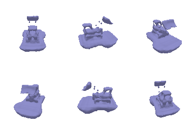
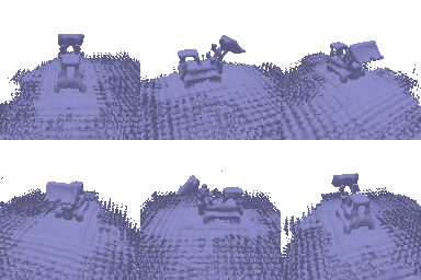
Chosen settings and why: α = 10, β = 0.01, eikonal weight 0.02, 250 epochs, plus sphere initialization. The network predicts a correction on top of the SDF of a radius-1 sphere, so training starts from a valid closed surface instead of noise. This fixes the main weakness of low β (no gradient when the surface starts in the wrong place). Low β can then deliver what it promises, the most accurate surface. It also removed the stray floor surfaces.
5. 3D Gaussian Rasterization
- 5.1 Projection:
- 3D covariance is
R S Sᵀ Rᵀ; for isotropic Gaussians it is simplys² I. - 2D covariance is
J W Σ Wᵀ Jᵀ, using the projection JacobianJand the camera rotationW. - 2D means come from projecting the 3D means to pixel coordinates.
- 3D covariance is
- 5.2 Evaluation: power is
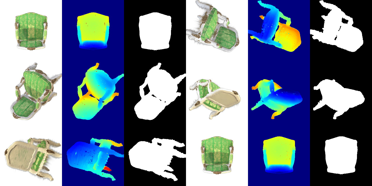
−½ (x−μ)ᵀ Σ⁻¹ (x−μ)for every Gaussian and pixel at once. All 4 unit tests pass. - 5.3 Sort and filter: Gaussians are sorted front-to-back by camera-space depth, and those behind the camera are dropped.
- 5.4 Alpha and transmittance:
alpha = opacity · exp(power). Transmittance is a cumulative product of(1 − alpha). - 5.5 Splatting: each Gaussian's weight is
alpha · T.- Color is the weighted sum of Gaussian colors.
- Depth is the weighted sum of Gaussian depths.
- The silhouette mask is the sum of the weights.
6. Training 3D Gaussian Representations
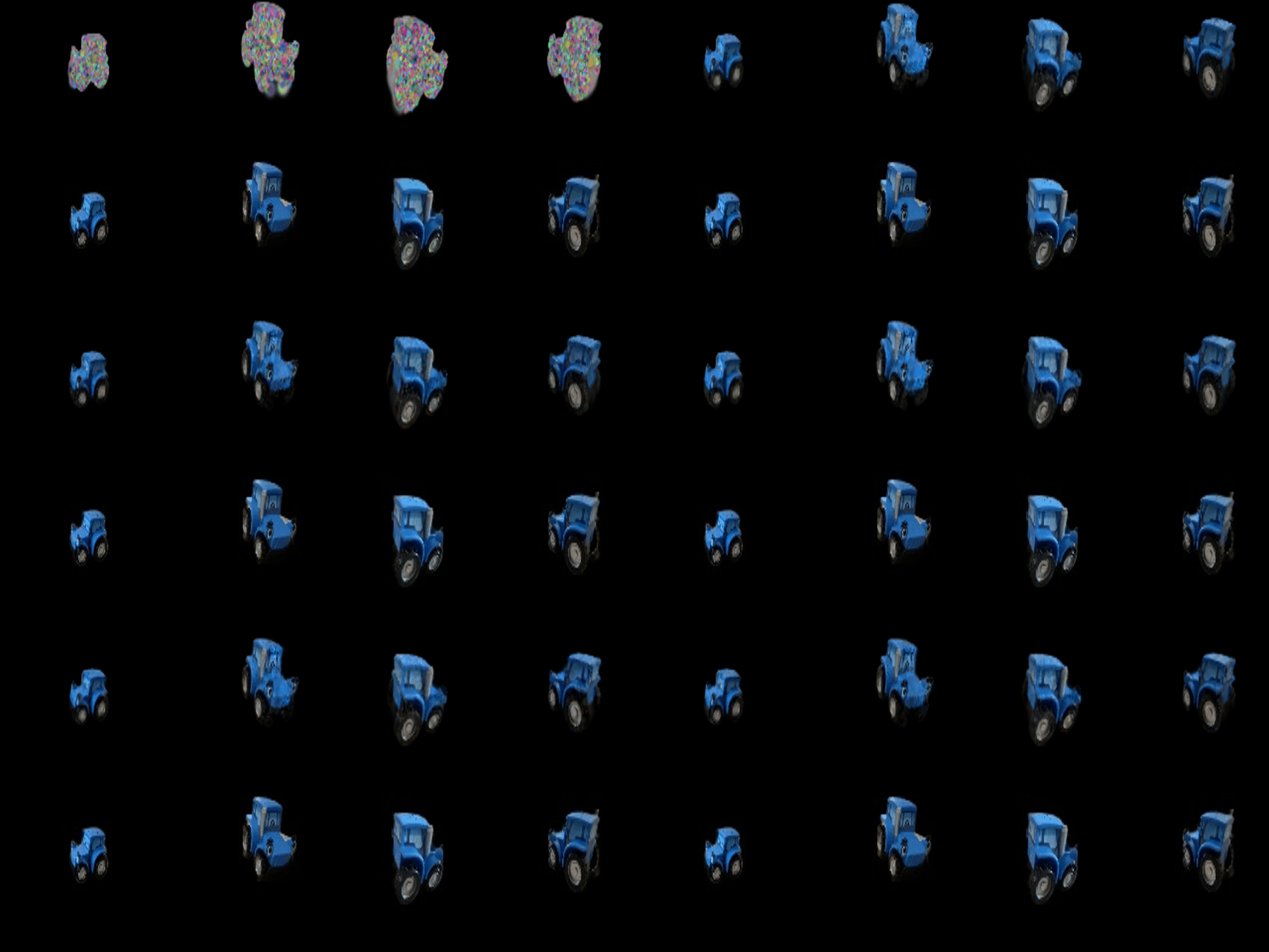
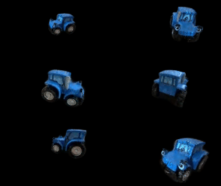
Isotropic Gaussians are initialized from the truck point cloud and trained with an L1 loss and Adam, using a separate learning rate for each parameter. Means get the smallest learning rate because small moves in position change the image a lot.
| Parameter | Learning rate |
|---|---|
| Opacities | 0.05 |
| Scales | 0.005 |
| Colours | 0.02 |
| Means | 0.0005 |
| Iterations | PSNR | SSIM |
|---|---|---|
| 1000 | 29.48 | 0.936 |
| 3000 (reported) | 30.78 | 0.948 |
7. Extensions (both done)
7.1 Rendering with spherical harmonics
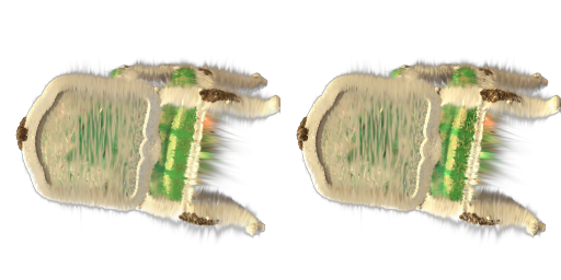
How: for each Gaussian we compute the direction from the camera center to its mean, then evaluate all 16 spherical-harmonic coefficients per color channel (degree 3) in that direction. This gives a color that depends on the viewing angle. Before, only the first, constant coefficient was used.
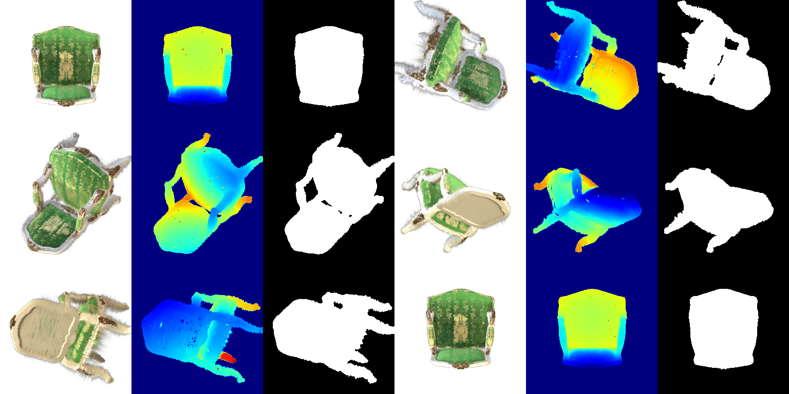
Side-by-side comparisons of the same views. Left: constant colour. Right: full spherical harmonics.


7.2 Training on a harder scene (materials, random init)
| Run | PSNR | SSIM |
|---|---|---|
| Baseline: Q6 setup, random init | 18.16 | 0.680 |
| + anisotropic, SSIM loss, longer training, LR decay | 18.70 | 0.713 |
| + wider random init | 23.08 | 0.853 |
| + wider init + densification | 23.73 | 0.880 |
| + init matched to scene bounds + densification (best) | 23.81 | 0.884 |
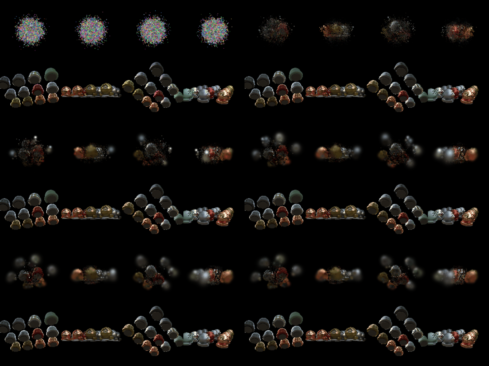
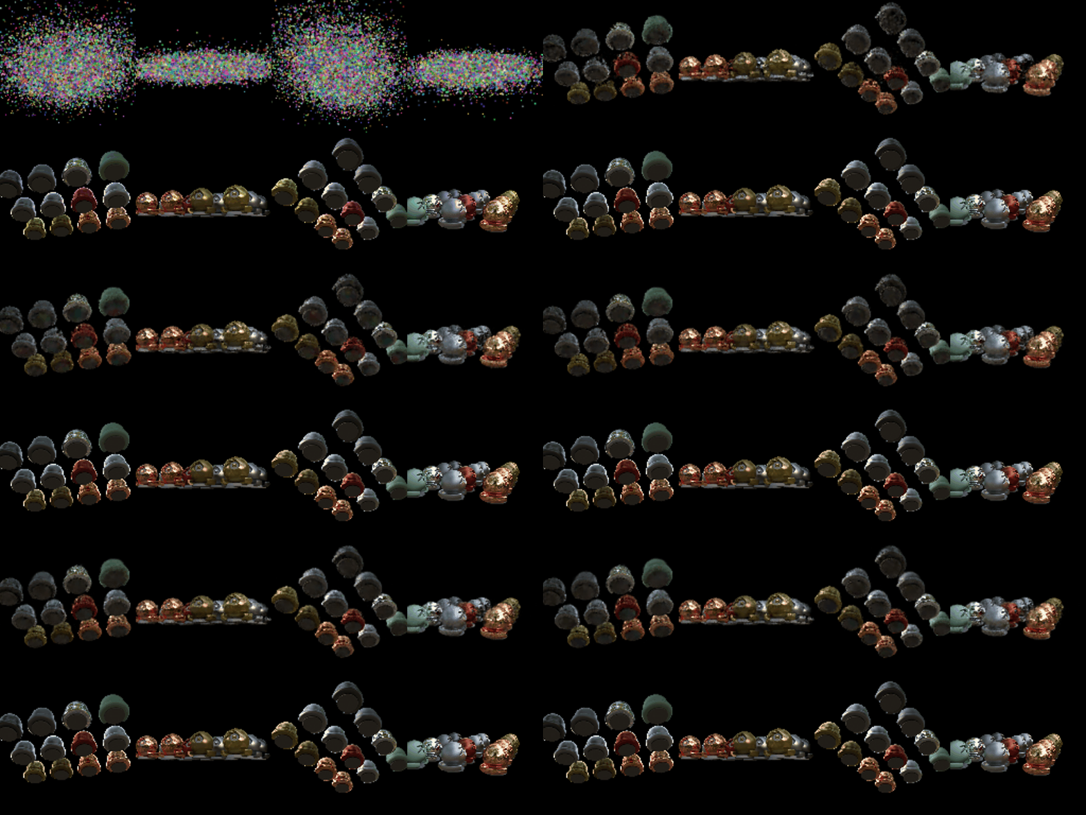
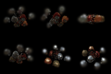

Changes from the Q6 setup (best run):
- Wider initialization (largest gain, ≈ +4.4 dB). The default random init puts every Gaussian in one small ball (std 0.2) at the center, but the materials objects are spread about 2 units wide. Spreading the points to match the scene (std 0.65, 0.55, 0.12 on x, y, z) lets Gaussians start near every object. We estimated these bounds from the density of our 4.1 NeRF. Using a plain std of 0.6 with no scene knowledge gets almost the same result: 23.73 / 0.880.
- Densification and pruning. Every 200 steps, for the first 60% of training:
- Gaussians with opacity below 0.005 are removed.
- The 10% with the largest position gradients are split into two smaller Gaussians.
- The total is capped at 25k Gaussians.
- Anisotropic Gaussians: rotations are learned too, so Gaussians can stretch to fit edges and flat surfaces.
- Loss: 0.8 · L1 + 0.2 · (1 − SSIM), as in the original paper. This favours sharp structure over blur.
- Learning rates: means start at 1e-3 and decay exponentially to 1e-5, so they move fast early and settle later.
- Longer training: 4000 iterations instead of 1000.
Without the wider initialization, the other changes gave only about +0.5 dB, even with 2× the Gaussians. The narrow initialization was the main bottleneck.