16-825 Assignment 2: Single View to 3D
Learning for 3D Vision · Abhikhya Tripathy (abhikhyt)
1. Exploring Loss Functions
Each GIF shows the Optimized shape on the left and the ground truth on the right.
1.1 Fitting a voxel grid
Details: voxel_loss is binary cross-entropy between the source grid and the binary target grid. The source grid is
Optimized as unconstrained logits (binary_cross_entropy_with_logits) and passed through a sigmoid before
marching cubes at 0.5 for the render.

1.2 Fitting a point cloud
Details: chamfer_loss is written with knn_points only: for every source point the squared distance to its
nearest target point, and for every target point the squared distance to its nearest source point, each averaged over
the points and summed.

1.3 Fitting a mesh
Details: The mesh is fitted with the Chamfer loss on points sampled from both surfaces plus smoothness_loss, a uniform
Laplacian smoothing term (weight 0.1) that keeps each vertex close to the average of its neighbours.

ico_sphere(4) (left) (2,562 vertices) and ground-truth mesh (right).I also tried two other initial meshes for the same target:

ico_sphere(2) (162 vertices): too few vertices to form the legs.
2. Reconstructing 3D from a Single View
--load_feat was not used. Checkpoints were saved every 10,000 iterations and all results below use the
90,000-iteration checkpoint. Each example is a turntable GIF with the input RGB on the left. F1 scores are averages over
the 678 test chairs.
2.1 Image to voxel grid
Decoder: a linear layer to a 256×4×4×4 volume, three transposed 3D convolutions (each doubling the resolution, with batch norm and ReLU) up to 32×32×32, and a 1×1×1 convolution that outputs occupancy logits. Trained with the binary cross-entropy loss from 1.1. Predicted and ground-truth voxels are shown as marching-cubes surfaces in the frame of the ground-truth mesh.
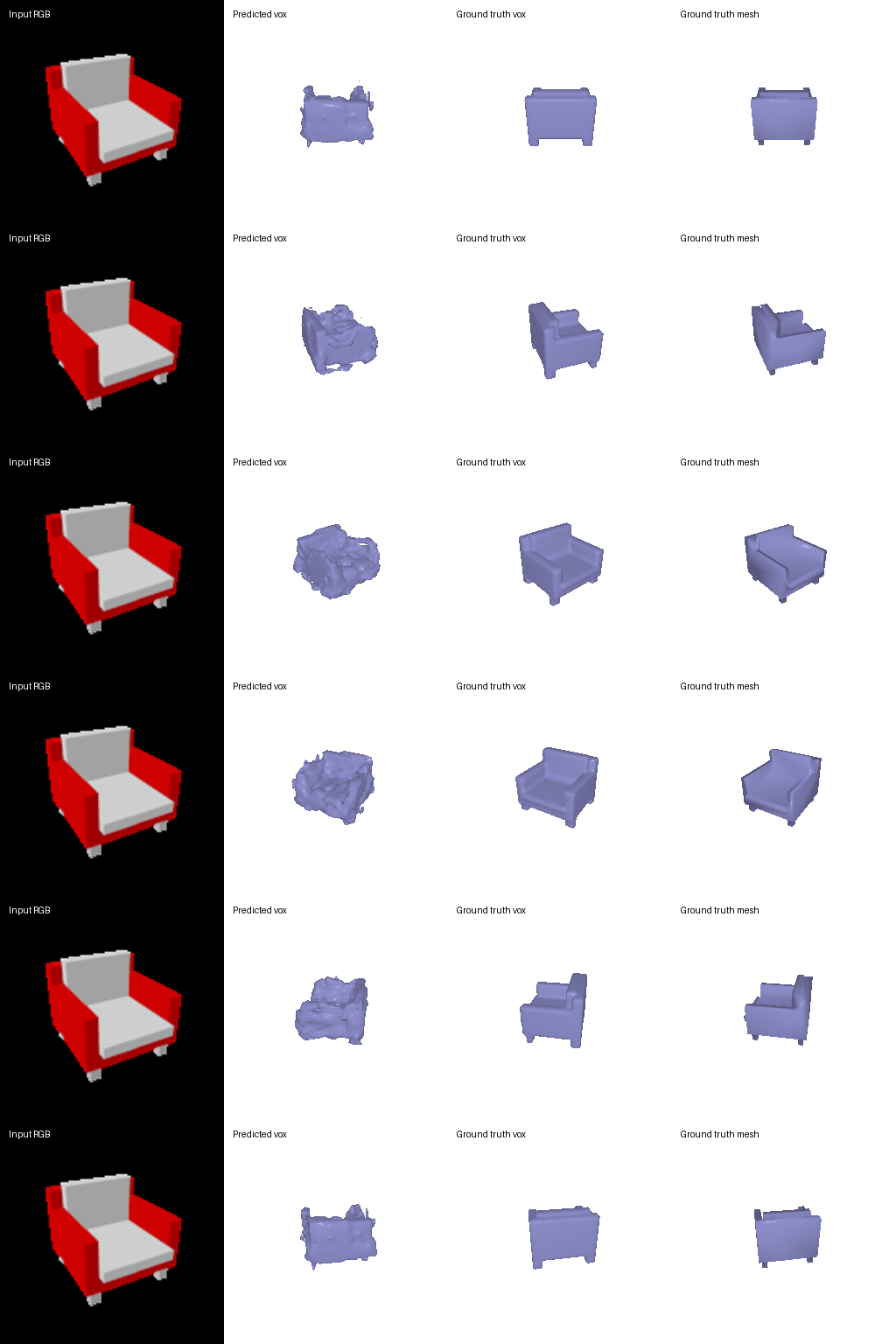
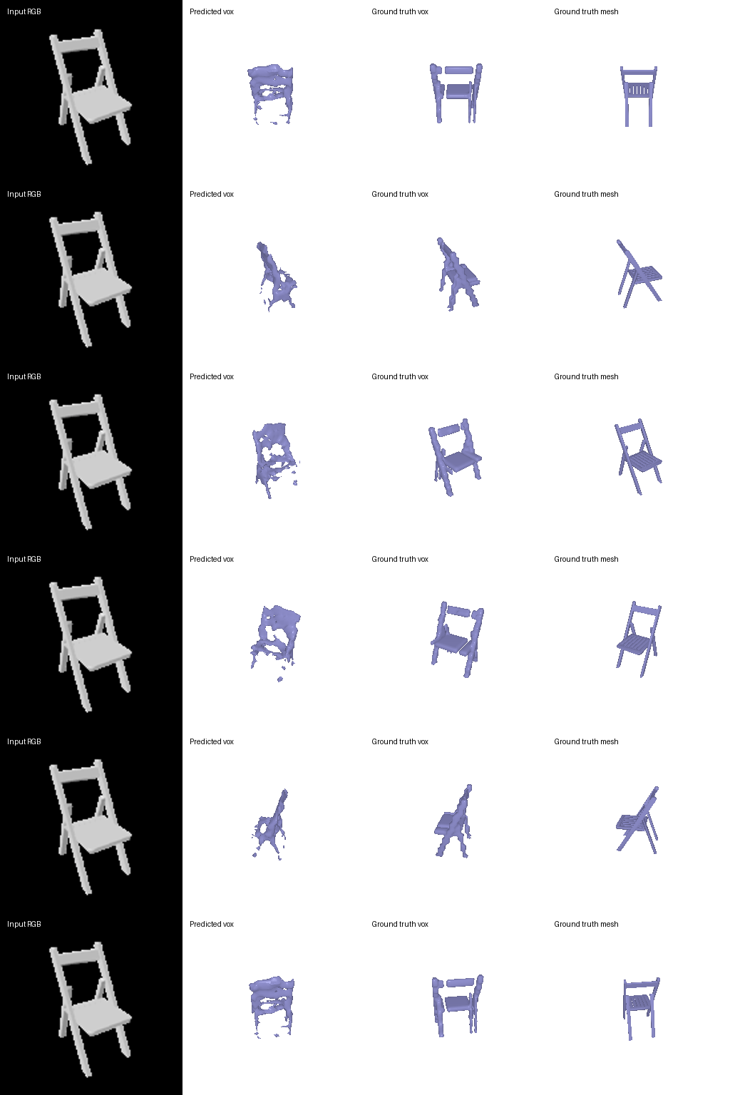
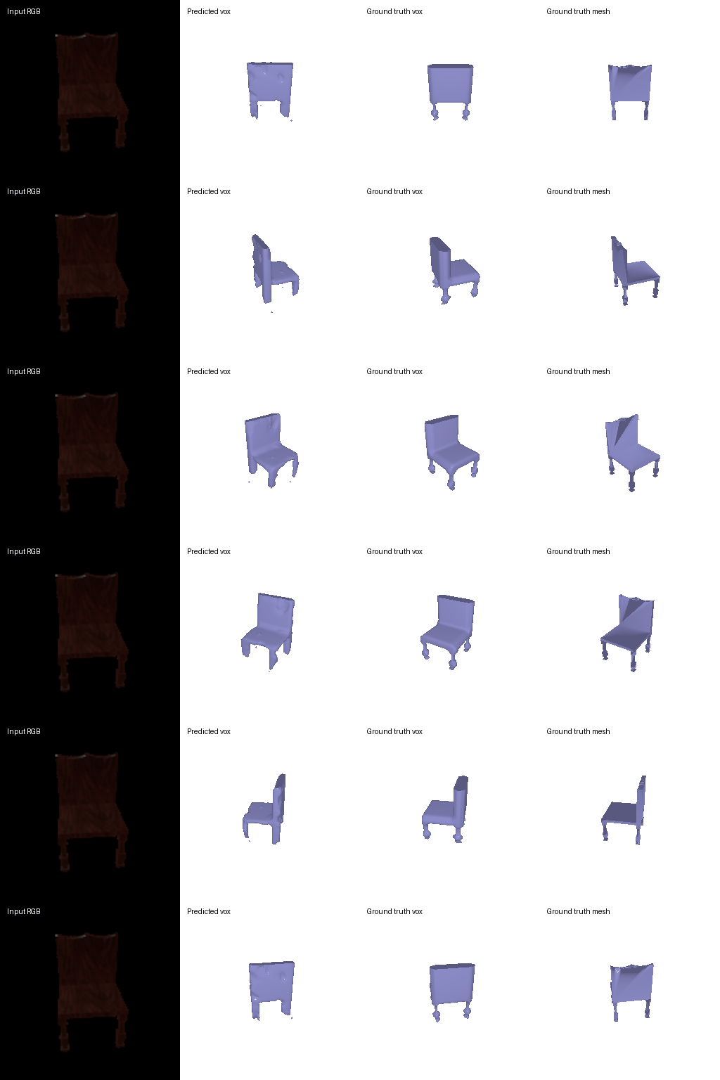
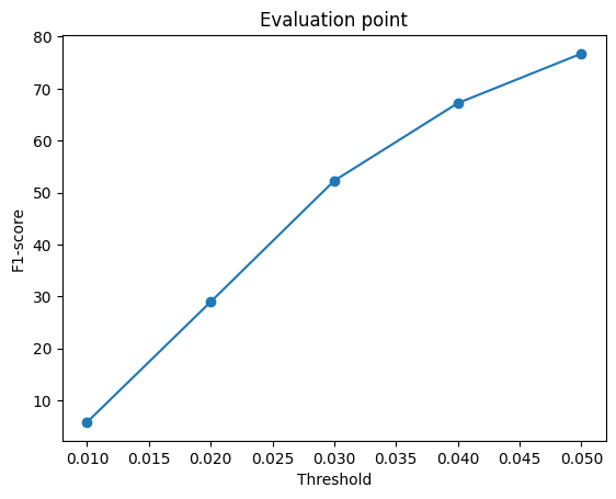
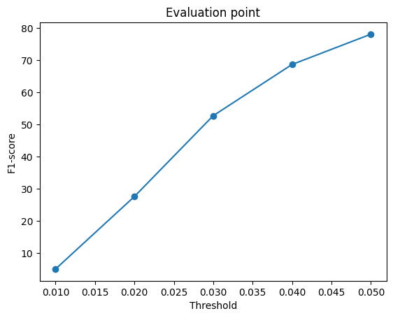
F1@0.05 = 76.0

2.2 Image to point cloud
Decoder: an MLP (512 → 1024 → 2048 → 3×1000) with a tanh on the output, giving 1,000 points. Trained with the Chamfer loss from 1.2 against 1,000 points sampled from the ground-truth mesh.
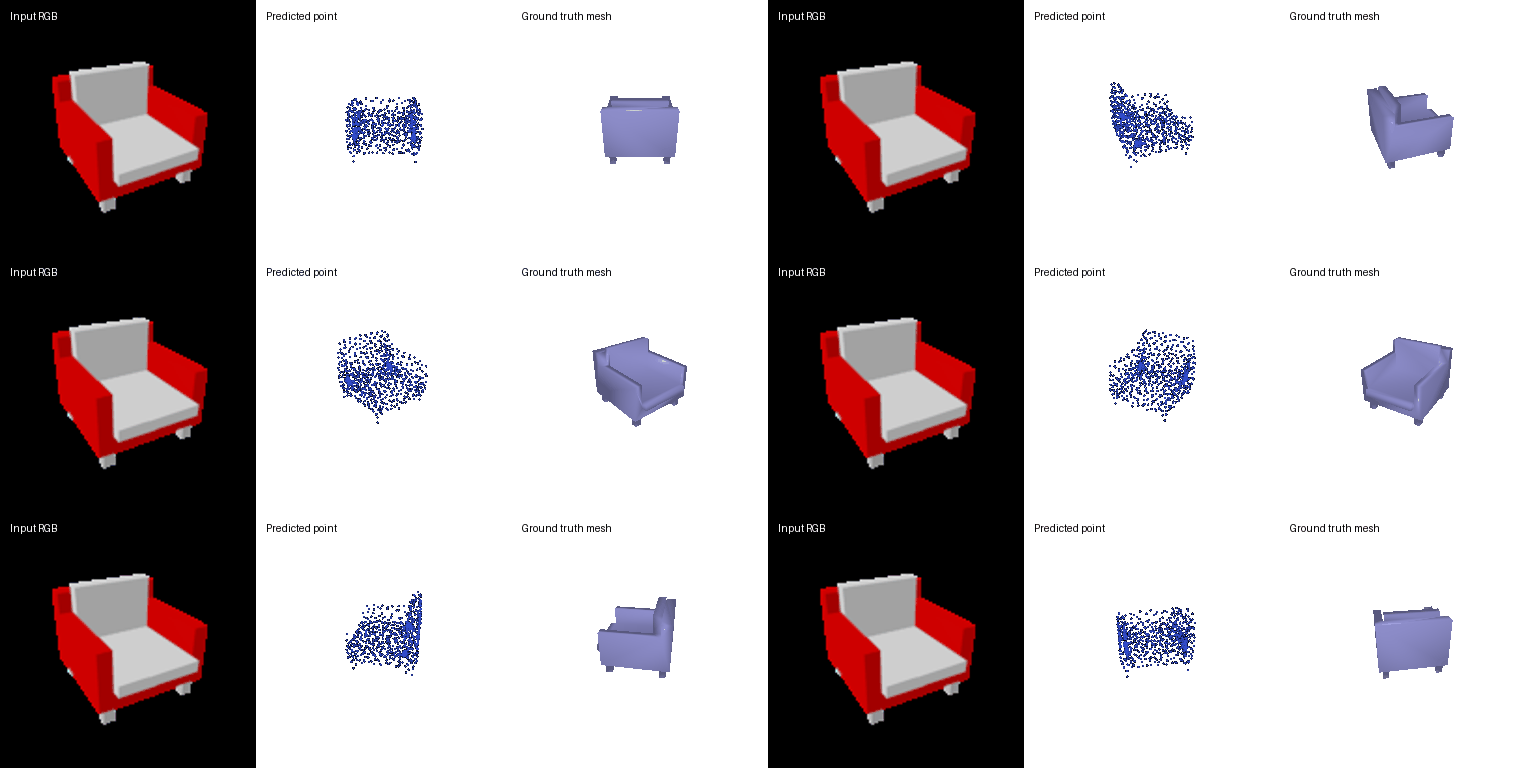
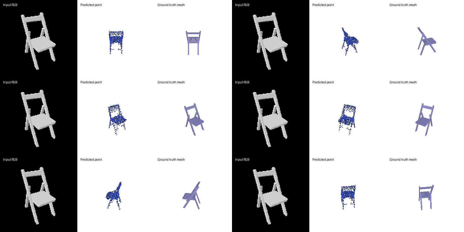
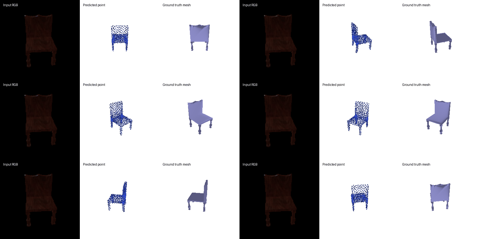
F1@0.05 = 76.7
2.3 Image to mesh
Decoder: an MLP (512 → 1024 → 2048 → 3×2562) that predicts one offset per vertex of an
ico_sphere(4) template. Trained with the Chamfer loss on 1,000 points sampled from each surface plus 0.1 × the
Laplacian smoothness loss from 1.3.
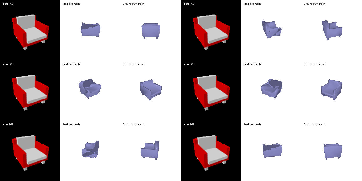
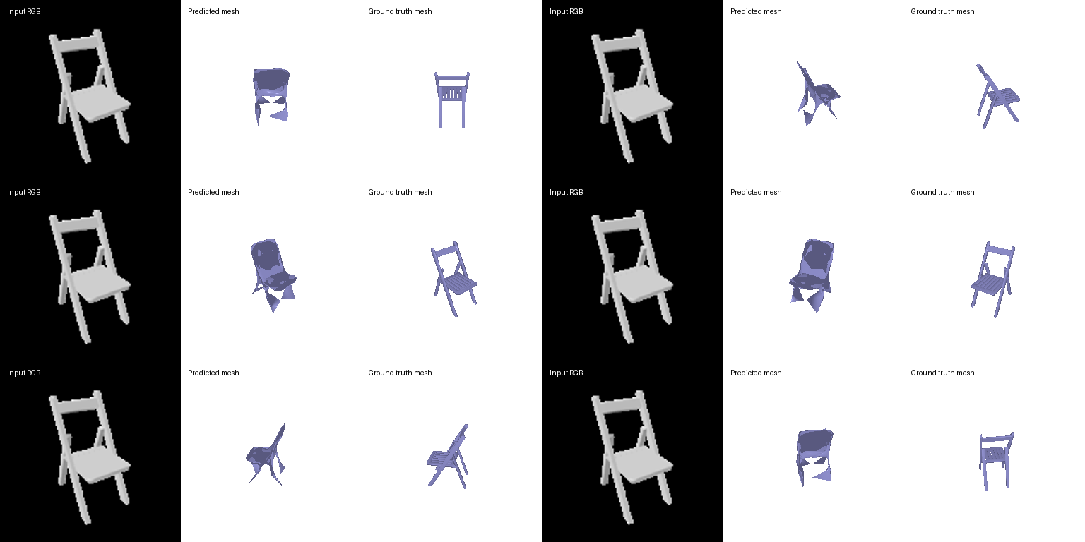
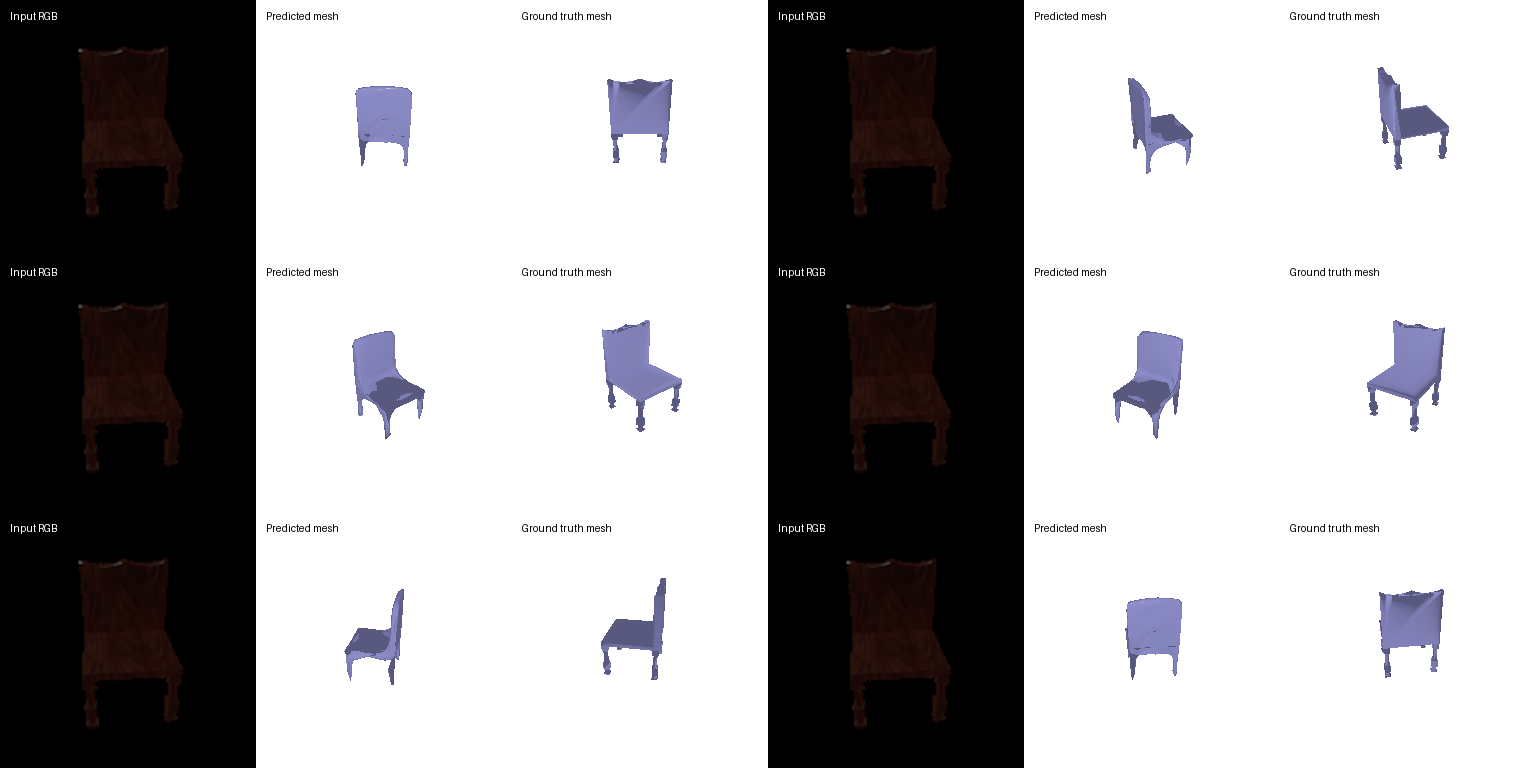
F1@0.05 = 72.7

Comparison of the three representations
| Representation | F1@0.05 |
|---|---|
| Point cloud (1,000 points) | 76.7 |
| Voxel grid (32³) | 76.0 |
Mesh (ico_sphere(4)) | 72.7 |
The point cloud scores highest, the voxel grid is close behind and the mesh is lowest. Point cloud is trained with the Chamfer loss which is a quantity that's very close to the F1 score (how many predicted points are near the ground truth and vice versa). The points also don't need to sit on a grid or follow any connectivity so they can sit on thin structures and create gaps wherever the shape needs that. So, the point cloud scores highest. Voxel grids are next because occupancy can handle varied topologies, including holes. However, the grid we used is coarse, so thin parts such as legs are often missing or fragmented at the 0.5 threshold. The mesh scores the lowest because the network deforms vertices of a sphere, so the output is always a single closed surface with no holes. Gaps get created by stretched faces and points sampled on such faces count as false positives. The smoothing loss also counters sharp edges and corners that thin structures might need.
2.4 Effect of the initial mesh (hyperparameter variation)
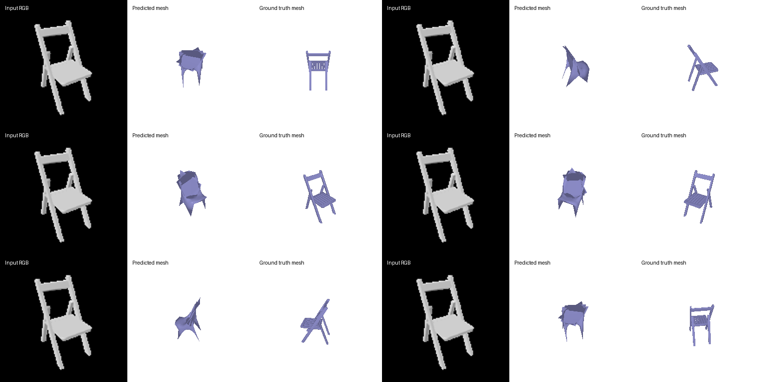
I varied the template mesh that the mesh decoder deforms, keeping everything else fixed (same losses and weights, 1,000 sampled points, 90,000 iterations). This changes two things: the number of vertices, and the topology.
| Template | Vertices | Topology | F1@0.05 |
|---|---|---|---|
ico_sphere(2) | 162 | sphere (no holes) | 70.7 |
ico_sphere(4) (baseline in 2.3) | 2,562 | sphere (no holes) | 72.7 |
ico_sphere(5) | 10,242 | sphere (no holes) | 74.2 |
| Torus (r = 0.2, R = 0.5) | 2,048 | one hole | 73.9 |
ico_sphere(2)ico_sphere(4)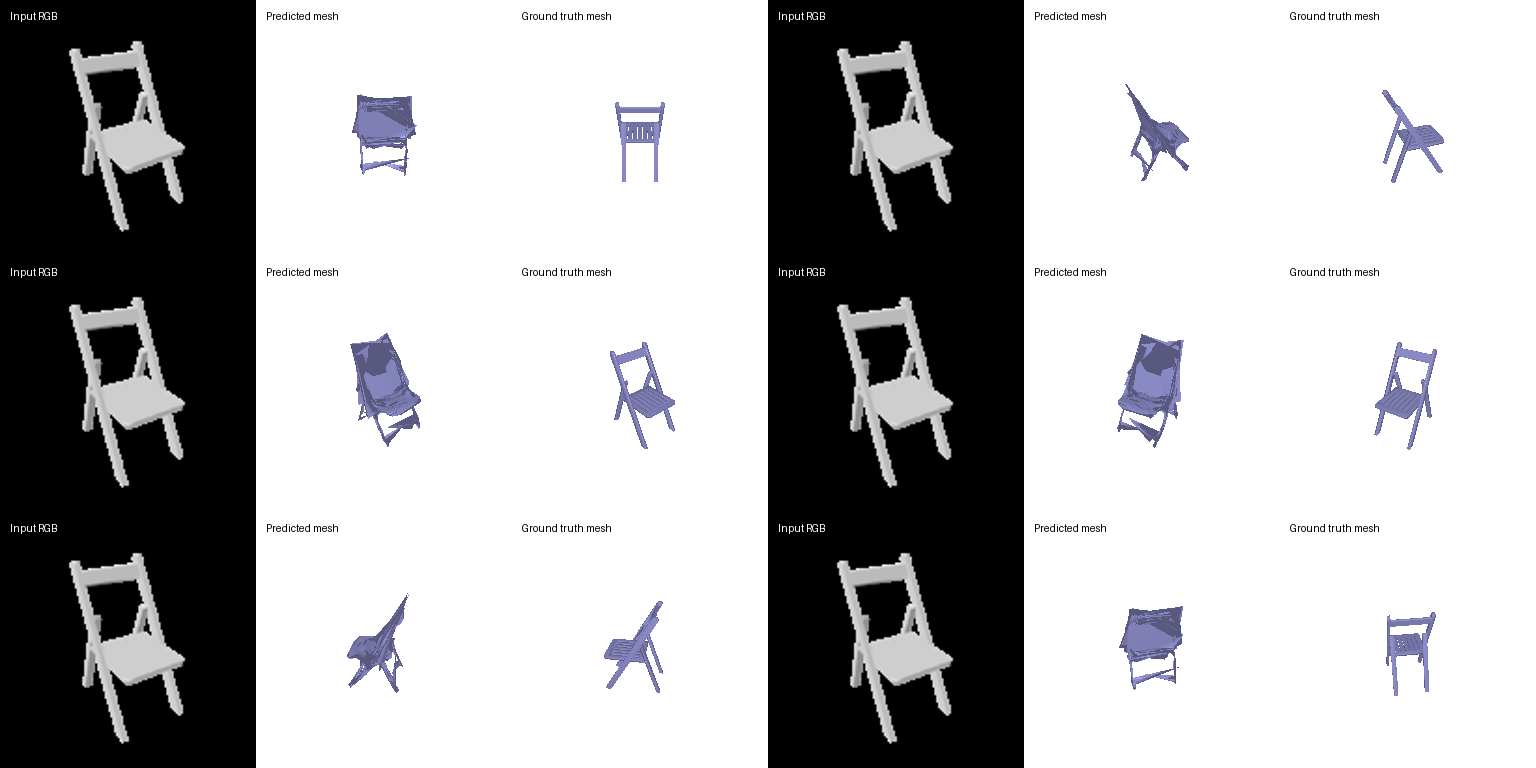
ico_sphere(5)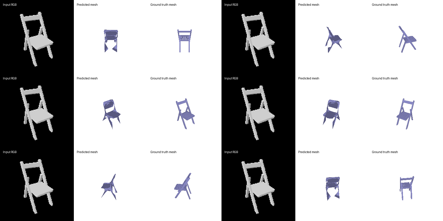
The same test image (test shape 200) given to each of the four models: input RGB, predicted mesh, ground-truth mesh. We observe the following:
- A higher number of vertices helps, but this gain saturates as the number of vertices increases too much. With 162 vertices for
ico_sphere(2)the mesh can only give the rough outline of the chair, with legs and arms needing more vertices for being expressed. - Topology of the starting mesh matters significantly. The torus scores higher despite having fewer vertices becasue its hole can be used for the opening in the back of the chair and the gap under the seat. We see that this starting mesh gives the cleanest output for those parts of the shape. A sphere tries to represent these parts only with stretched faces.
2.5 Interpreting the models
Two experiments, each run on the same test images for every model so the results can be compared.
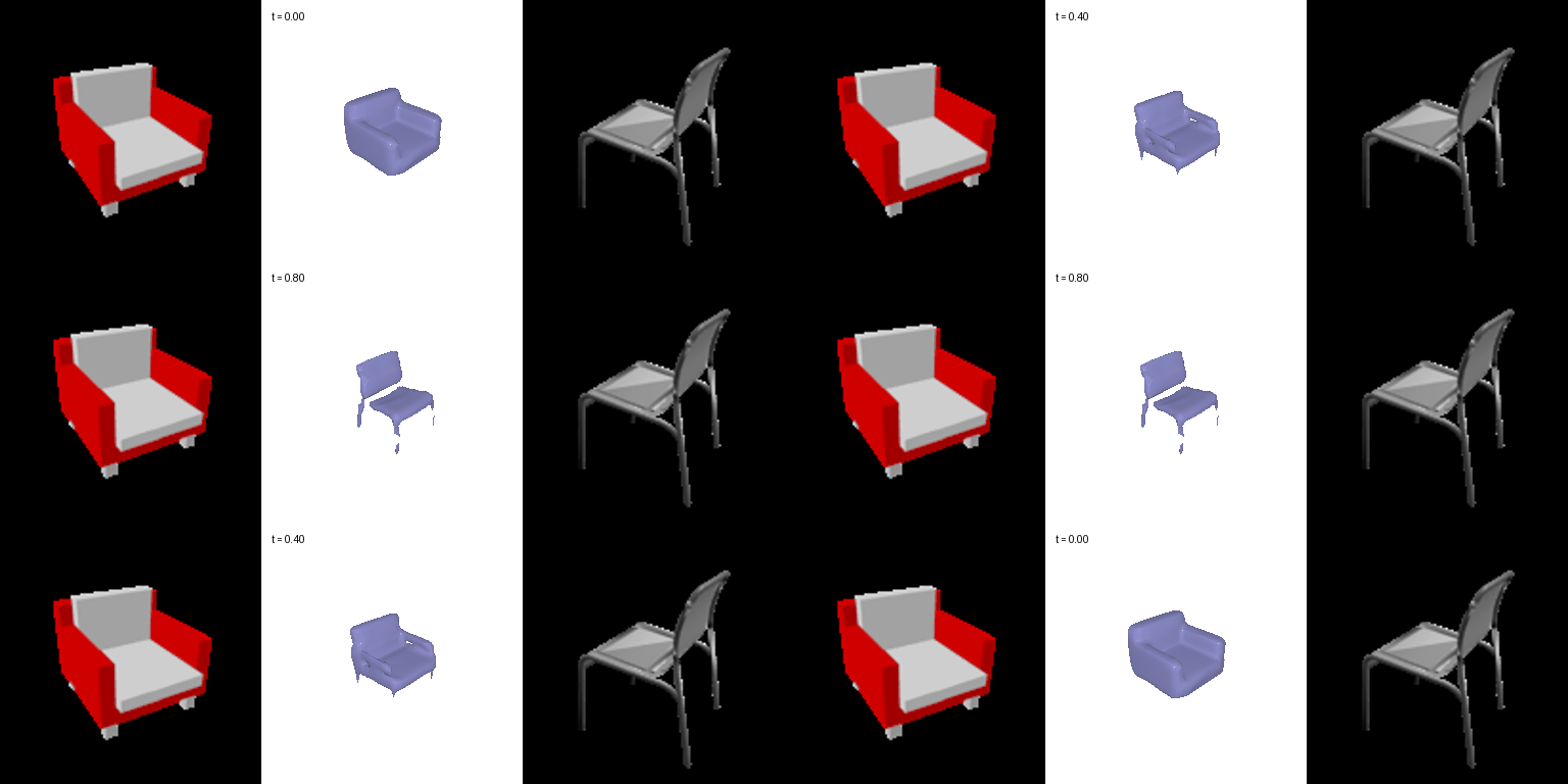
(a) Latent interpolation: is the shape space continuous?
The 512-d image features of two test images are blended linearly and every blend is decoded (inspired by Achlioptas et al.,
2018). A smooth morph means the decoder has learned a continuous space of chairs. t is the blending amount between the two input images, from 0 to 1: at t = 0 the shape is decoded purely from image A's feature, at t = 1 purely from image B's, and so on.
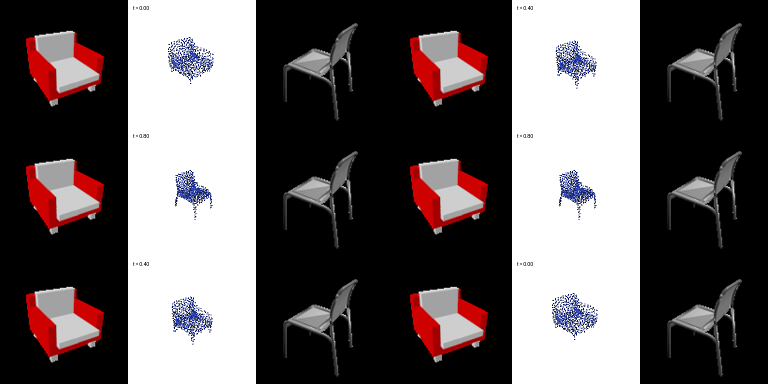
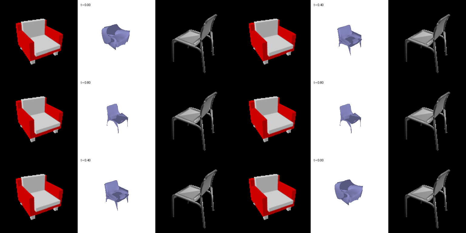


The point cloud and the mesh morph smoothly from the armchair to the thin chair: the arms shrink and the legs grow, with a plausible chair at every step. The voxel model does not. Its intermediate predictions break into scattered fragments, because the blended features give occupancies close to the 0.5 threshold. So the voxel decoder is confident at the two ends but not in between. It likely does not learn a continuous shape space for chairs.
(b) Checkerboard occlusion: how much does the model rely on seeing the full image?
Half of the input image is blacked out with a checkerboard of 8, 16 or 32 pixel cells, and compared with the clean image and with a completely black image (which shows what the model predicts when it sees nothing).


- Every model has a memorised default chair which it outputs when given a fully black image.
- Point cloud and mesh models degrade more smoothly. With half the image hidden, they still seem to be using the visible half effectively enough to generate a plausible chair that is different from the memorised chair and matches the input image to an extent.
- The voxel model however breaks down. This failure is aligned with the one seen in the latent interpolation experiment.
3. Exploring Other Architectures / Datasets
3.1 Implicit network
The implicit decoder takes the image feature and a 3D coordinate and outputs the occupancy of that single location. The coordinate and the 512-d feature are each projected to 256 dimensions and added, followed by a three-layer MLP that outputs one logit. To produce a full prediction it is evaluated on a 32×32×32 grid of coordinates in (-1, 1)³, so it is trained and evaluated exactly like the voxel model in 2.1 (same loss, same ground truth). The only difference is that one small network is shared across all locations instead of generating the whole grid at once.
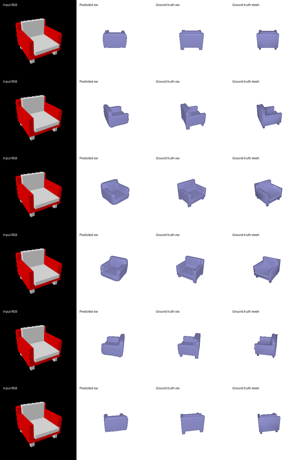
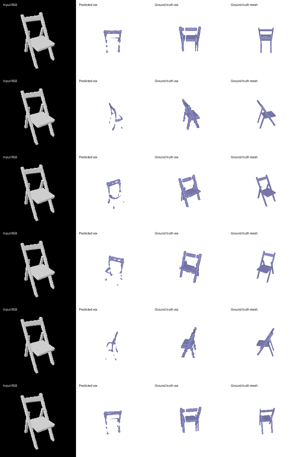
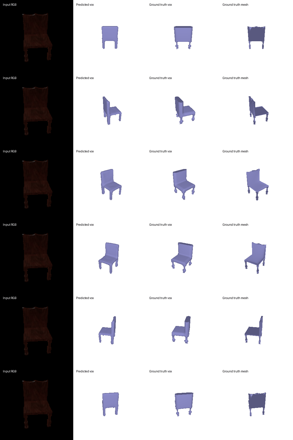
F1@0.05 = 74.2 (voxel decoder in 2.1: 76.0)
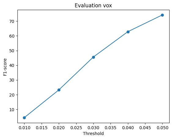
- Score. The implicit decoder scores slightly below the voxel decoder at the same 32³ resolution. A large part of this gap comes from the fact that for 15 of the 678 test shapes it predicts no occupied cell at all (probability below 0.5 threshold) and we score these as F1 = 0. On the remaining shapes, its average is 75.9.
- Shape quality. Its surfaces are smoother and more solid than the voxel decoder's. Occupancy is a continuous function of the 3D coordinate, so neighbouring cells get similar values. The same property shows in the interpolation: the implicit decoder morphs between two chairs without falling apart, unlike the voxel decoder in 2.5a.
- Weakness. Thin parts such as legs tend to be dropped, since a small MLP conditioned on one global feature favours smooth, low-frequency shapes.
- The decoder has far fewer parameters than the transposed-convolution decoder and, because it takes coordinates as input, it could be queried at any resolution without retraining.
3.2 Parametric network
The parametric decoder maps a 2D point sampled from the unit square, together with the image feature, to a 3D point
(a single-patch AtlasNet). The 2D point and the feature are each projected to 512 dimensions and added, followed by a
three-layer MLP with a tanh output. During training 1,000 random 2D points are sampled per image and the output is trained
with the Chamfer loss, exactly like the point model in 2.2.
- Score. The parametric decoder scores a little below the plain point decoder of 2.2. It has to produce every point as a continuous function of a 2D coordinate, i.e. the whole chair is one folded sheet, whereas the plain decoder regresses 1,000 independent points and can place each one freely.
- The number of output points is not fixed. The figure uses a 64×64 grid (4,096 points) from a model trained with 1,000 random points per image, which the plain point decoder cannot do.
3.3 Extended dataset for training
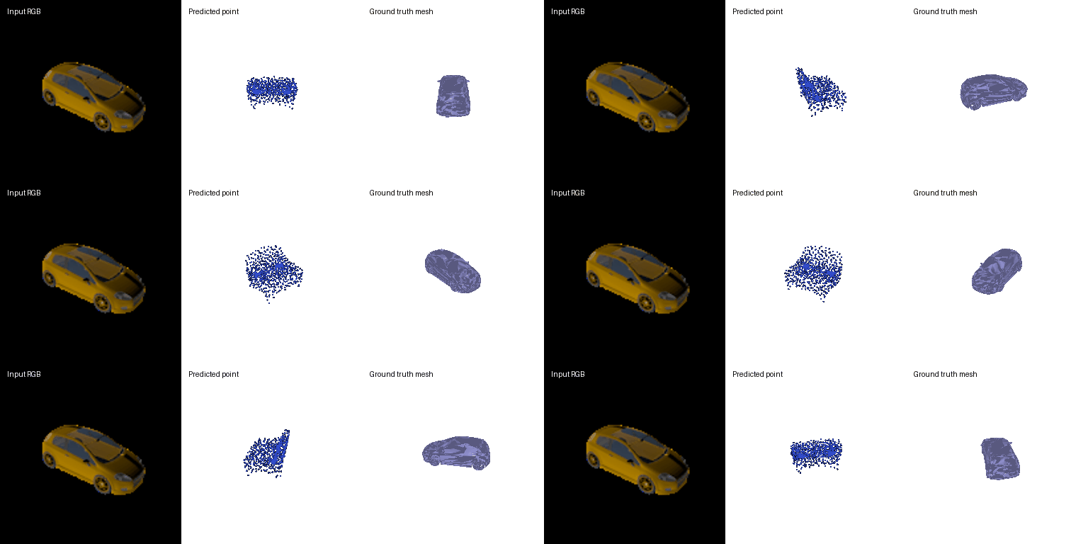
The point cloud model of 2.2 was trained on the three-class dataset (chairs, cars and planes; 12,886 training shapes) with the same settings and number of iterations, and compared with the model trained on chairs only.
| F1@0.05 of the point model | Chairs (678) | Cars (368) | Planes (405) | All three (1,451) |
|---|---|---|---|---|
| Trained on chairs only | 77.0 | 66.0 | 64.9 | 70.8 |
| Trained on three classes | 77.7 | 92.7 | 95.7 | 86.5 |
Scores vary by a few tenths between evaluation runs, because each run uses a randomly chosen view of every test shape.
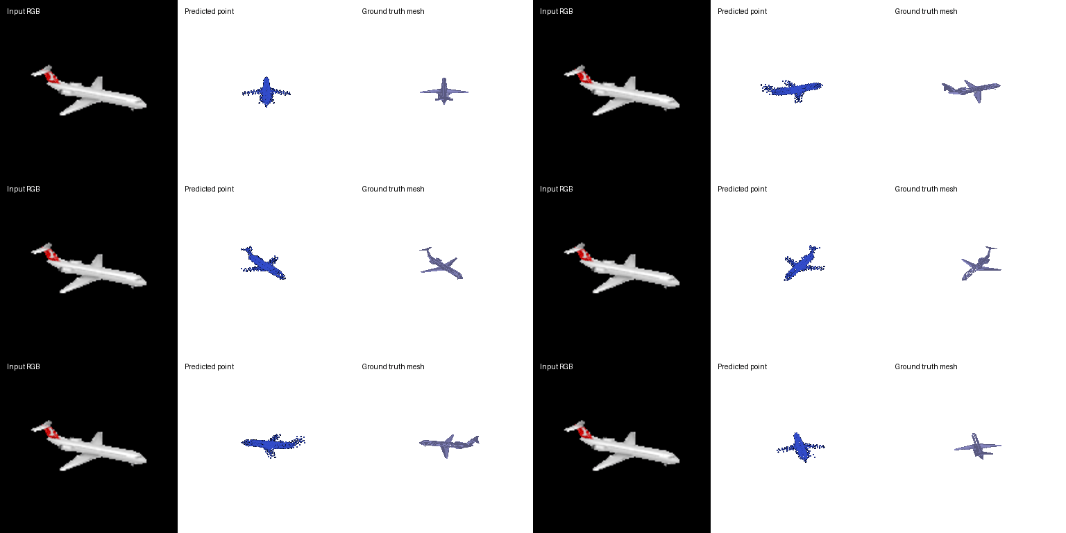
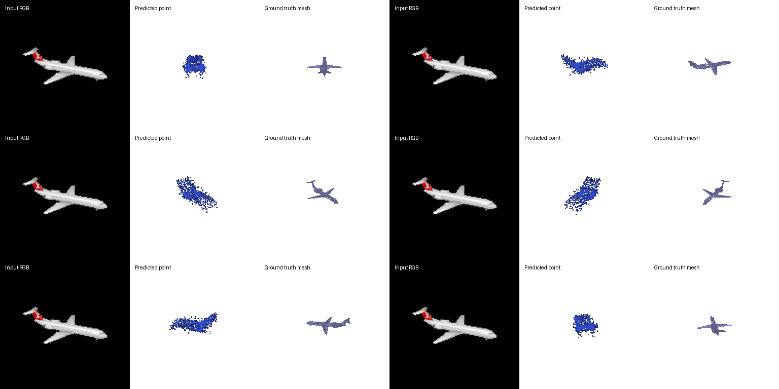
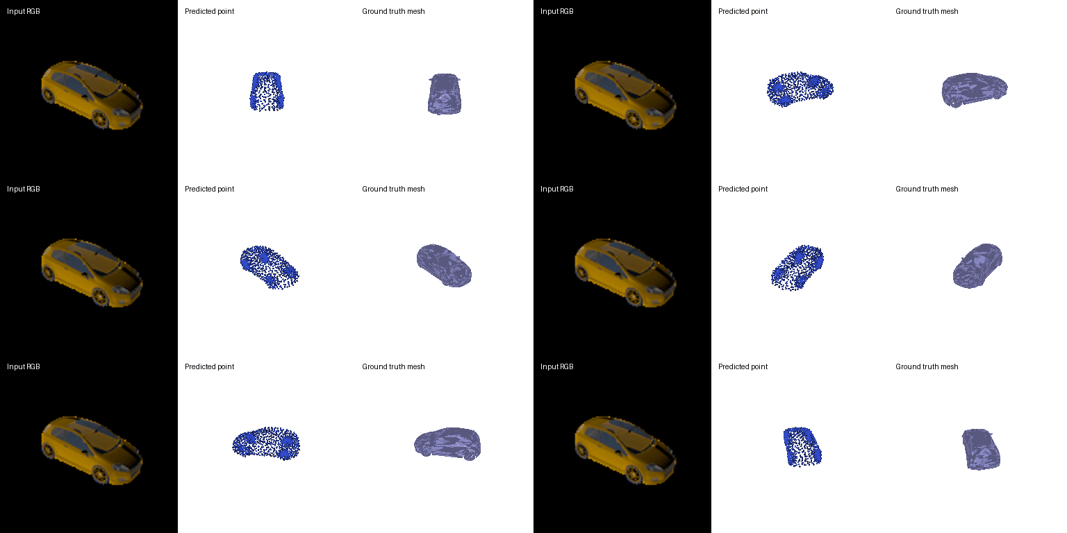
Same test image for both models
Each GIF shows the input RGB, the predicted point cloud and the ground-truth mesh.
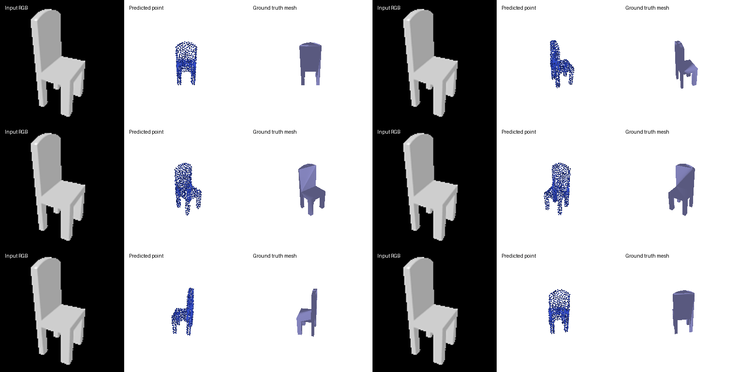
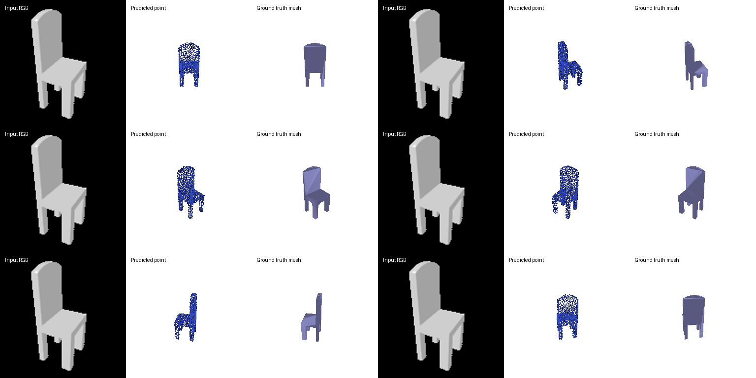
- Chairs: no loss from adding classes. On the same 678 test chairs the three-class model is at least as good as the chair-only model.
- Cars and planes: the chair-only model fails. It scores about 65 on both classes it never saw, against 93 to 96 for the three-class model. In the examples it turns a plane or a car into a compact blob of roughly the right size but with no wings or car body, so it can only produce outputs from the chair shapes it has learned.
- Consistency and diversity. The three-class model's outputs are more diverse overall, since it first has to recognise the class and then produce a class-specific shape, and its outputs within a class are consistent with the input. The chair-only model is consistent in a different way, whatever the input, it produces something from its space of chairs.