Assignment 2 : Gradient Domain Fusion
Poisson Blending: Mathematical Framework
The Poisson blending process involves solving an optimization problem that aims to blend the source and target images seamlessly. The optimization function can be described as follows:
v = argminv Σi∈S,j∈Ni∩S ((vi - vj) - (si - sj))2 + Σi∈S,j∈Ni∩¬S ((vi - tj) - (si - sj))2
vrepresents the pixel values in the blended image we are trying to find.Sis the set of pixels in the source image's region we wish to blend.Niis the set of neighboring pixels around pixeli.viandvjare the pixel values in the blended image at positionsiandj, respectively.siandsjare the pixel values in the source image at positionsiandj, respectively.tjis the pixel value in the target image at positionj.¬Srepresents the region outside ofS, the complement of the source region.
- The first term ensures that the difference in gradients between neighboring pixels within the source region in the blended image (
vi - vj) is similar to that in the source image (si - sj). - The second term ensures that the pixel values at the boundary of the source region in the blended image match the corresponding pixel values in the target image, allowing for a seamless transition.
Toy Problem
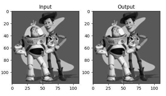
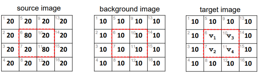
The toy problem in gradient domain processing is a fundamental technique used to understand how to manipulate image gradients for tasks like image blending. It involves calculating the gradients in the x and y directions from a source image and using these gradients to reconstruct an image.
The source image is denoted by s(x,y) and the target image by v(x,y). The task is to solve for v(x,y) such that it maintains the gradient of s while also adhering to certain constraints.
- Minimize the difference in x-gradients between v and s which can be written as v(x+1, y) - v(x, y) \approx s(x+1, y) - s(x, y) .
- Minimize the difference in y-gradients between v and s written as v(x, y+1) - v(x, y) \approx s(x, y+1) - s(x, y) .
- Ensure the top left corners of v and s have the same color, adding the constraint v(1, 1) = s(1, 1).
These constraints are set up as a least squares problem which can be mathematically represented and solved using linear algebra. The least squares approach will find the pixel values for image v that best fit the gradient constraints taken from image s. The implementation involves setting up a system of equations Av = b, where A is a matrix representing the gradient constraints, v is the vectorized form of the image to be solved, and b is a known vector derived from the gradients of s. This system can be solved using numerical methods such as the least squares solver in NumPy's linear algebra package. Once you solve for v, you can reshape this vector back into the form of an image and see if the reconstructed image v matches the original source image s. If the reconstruction is correct, you will have effectively demonstrated how to manipulate and reconstruct images in the gradient domain.
Poisson Blending
The overall process of Poisson Blending is as follows:
- Preparation of the Mask: Convert the mask to a boolean array to indicate which pixels to blend.
- Mapping Pixels to Variables: Each pixel within the mask is mapped to a variable in a linear system.
- Setting Up the System of Equations: A sparse matrix system is created to solve for pixel values.
- Calculating the Divergence: The divergence of the gradient at each pixel is calculated and set in the system.
- Boundary Conditions: Target image values are used for boundary pixels to ensure a seamless blend.
- Solving the Linear System: The sparse system is solved to find the optimal blended pixel values.
- Reconstructing the Image: The solved pixel values are inserted back into the target image.
- Result: The final blended image with a smooth transition is produced.
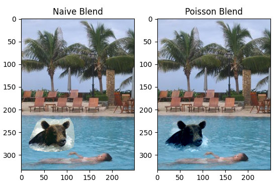
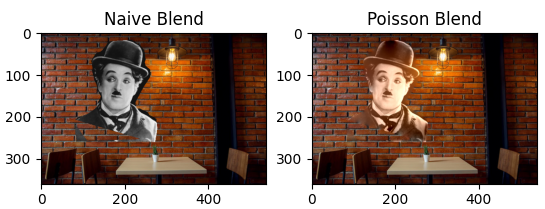
Some of the results are as follows:
Example Image
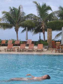
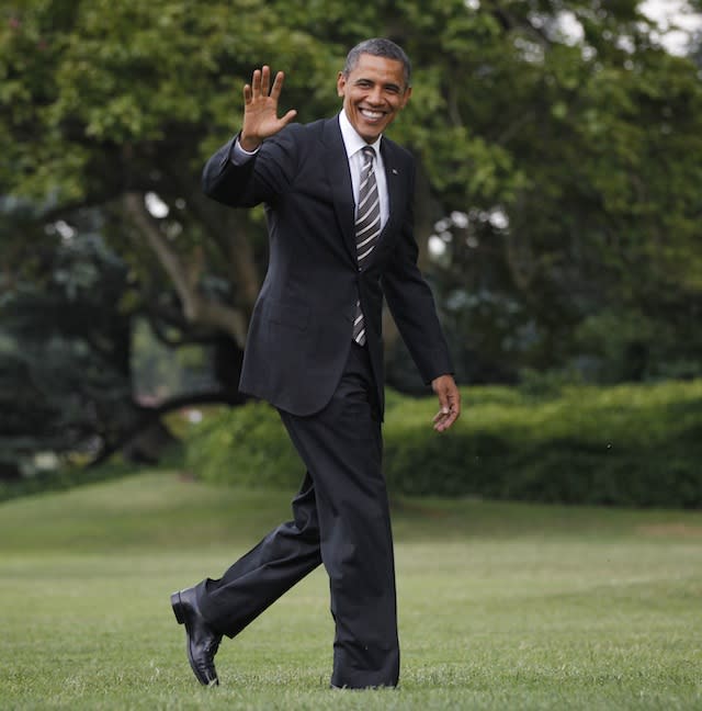
Source Image
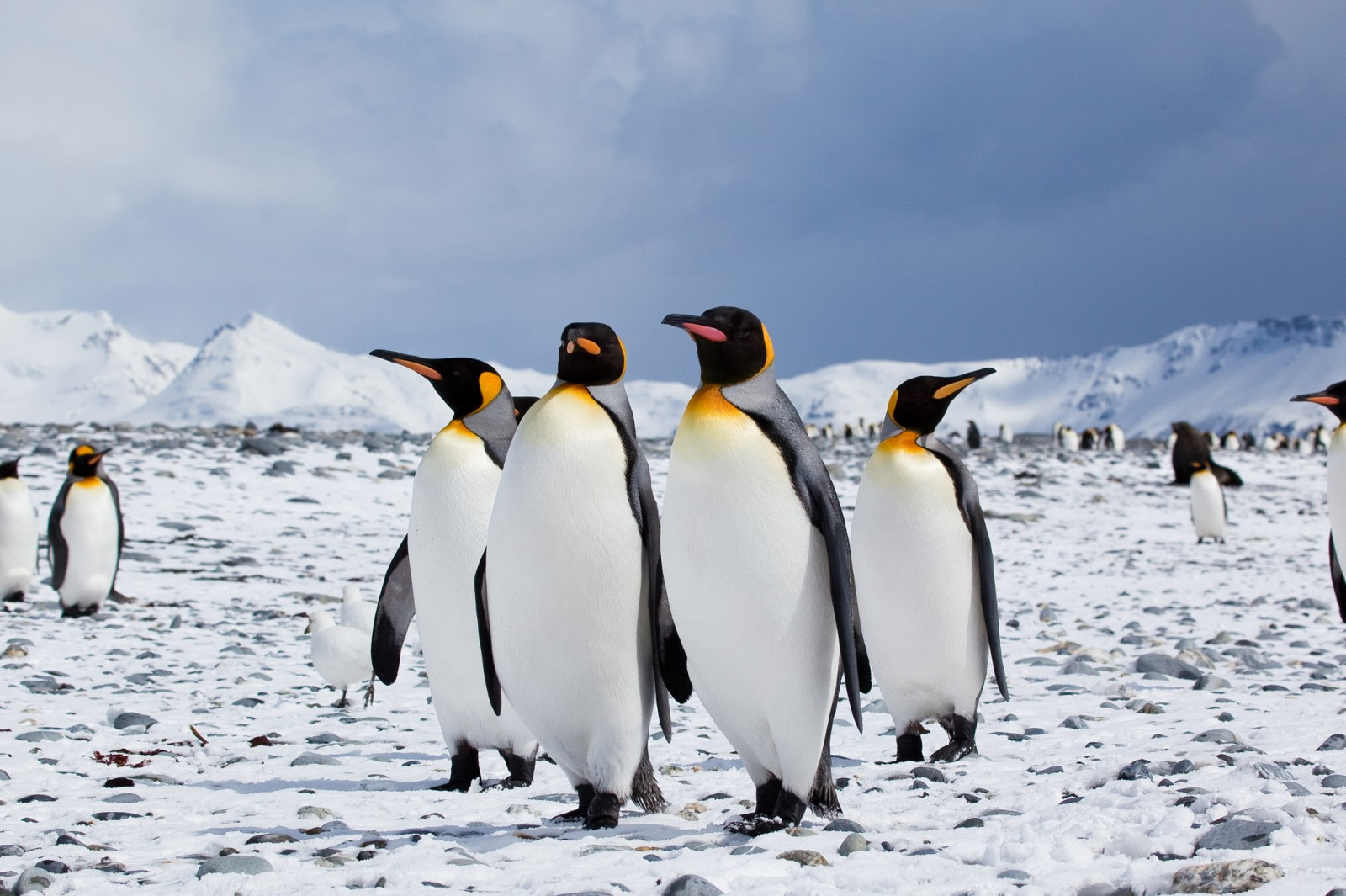
Target Image
Favorite Image
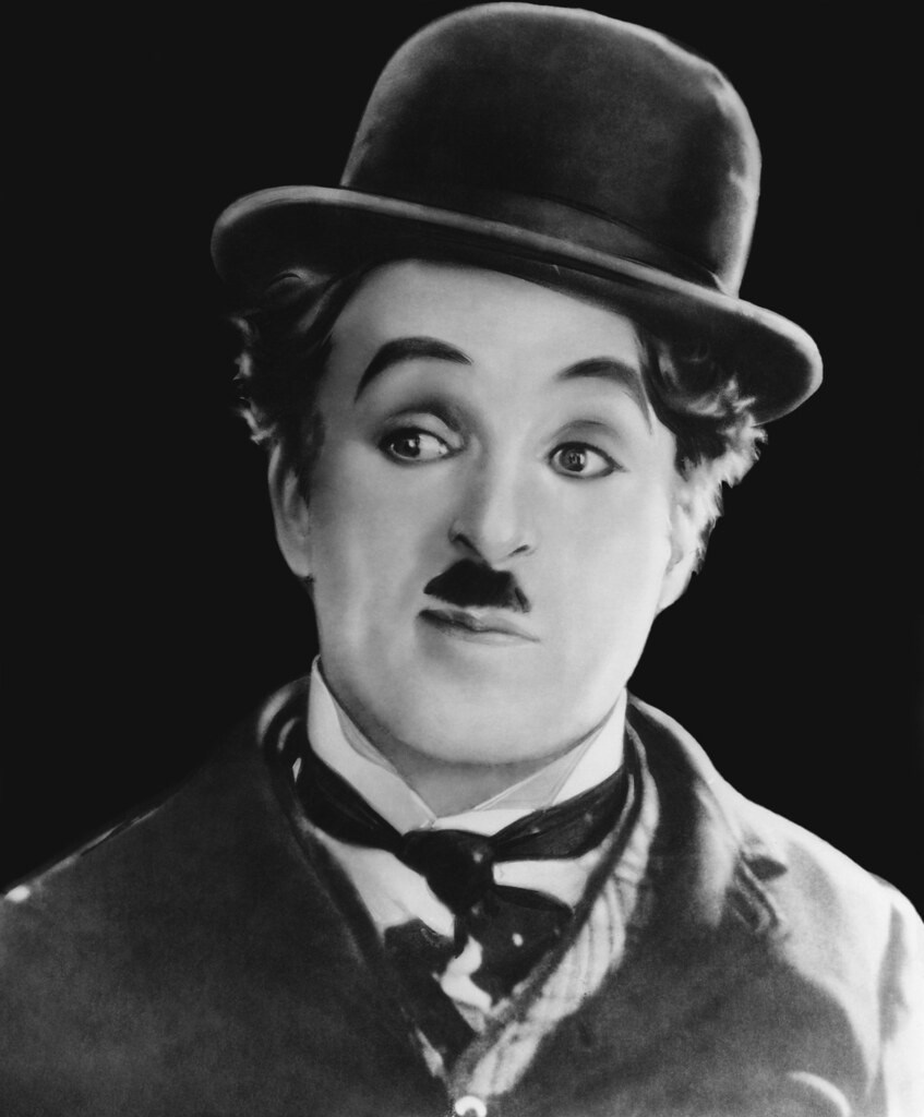
Source Image
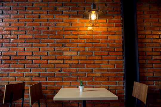
Target Image
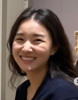
Source Image
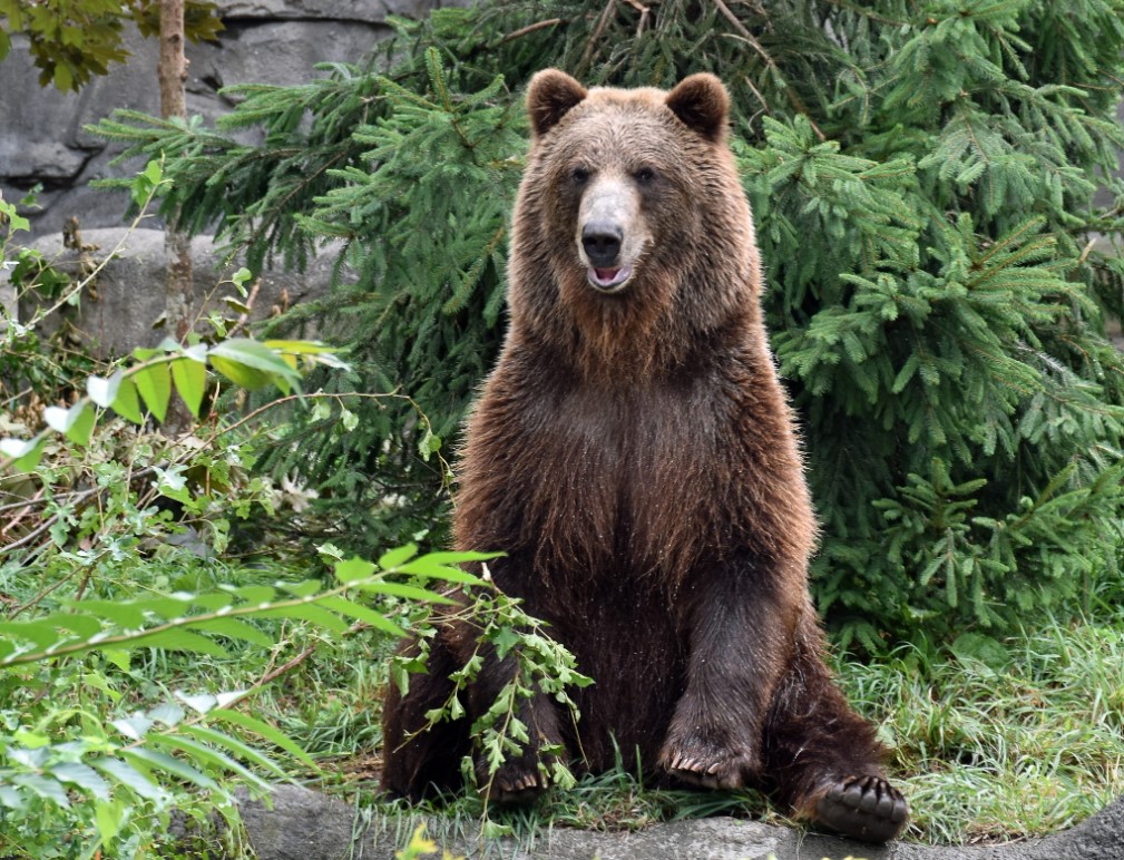
Target Image
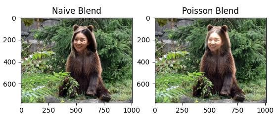
Failed Image
Source Image
Target Image
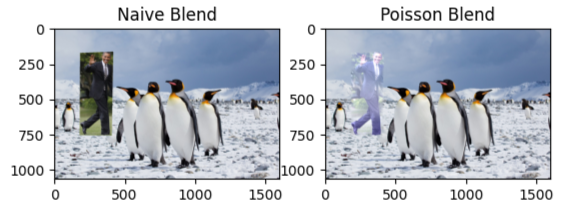
Unsuccessful Poisson Blending: Potential Causes
Several factors could contribute to the unsuccessful blending observed in Poisson Blending:
- Incorrect Masking: Poisson blending requires an accurate mask that defines the region of the source image to be blended. If the mask is not correctly defined, the algorithm may not interpret which gradients to match correctly, leading to a poor blend.
- Gradient Mismatch: The Poisson algorithm relies on the assumption that the gradients of the source and target can be matched smoothly. Significant differences in gradient fields due to lighting or texture might prevent the algorithm from finding a solution that blends the images naturally.
- Boundary Conditions: If boundary conditions are not correctly enforced or if the region where the source and target meet is not well-defined, the algorithm may fail to produce a result that aligns well with the target image.
- Image Content and Complexity: The content of the images being blended can affect the outcome. Blending a complex object into a complex background may not be as seamless as blending a simple object into a uniform background.
- Algorithm Limitations: Poisson blending may struggle with scenarios where there is a vast difference in color intensity ranges between the source and target images, potentially causing blending artifacts or color distortions.
Mixed Gradient Belnding
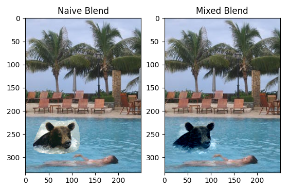
Mixed Gradients Blending is an image processing technique that refines the concept of Poisson blending by selectively using the largest gradient magnitude from either the source or the target image to guide the blending process.
The process aims to minimize the squared differences between the blended image gradients and the larger gradients from the source or target. The mathematical expression is as follows:
v = argmin_v ∑ (|∇v - d_ij|)^2
where d_ij is the gradient chosen from the source or the target image at each pixel.
The selection of gradients is based on their magnitude, favoring the gradient that has the higher magnitude between the source and target images. This decision is made for each pixel, ensuring that the most dominant features are preserved in the blending process.
if abs(∇s_i - ∇s_j) > abs(∇t_i - ∇t_j):
    d_ij = ∇s_i - ∇s_j
else:
    d_ij = ∇t_i - ∇t_j
This technique provides several benefits:
- It preserves sharp features and ensures smooth transitions by selectively choosing gradients.
- The blending often appears more natural by accommodating texture and lighting variations.
- It's particularly effective when blending images with plain backgrounds into more textured scenes.
Mixed Blend result:
Color2Gray
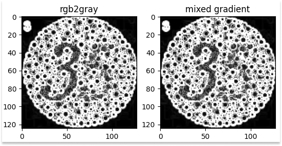
Converting color images to grayscale is a common process, but standard methods like MATLAB's rgb2gray can result in the loss of important contrast information. This makes details harder to distinguish, particularly when the image is used in different contexts, such as printing.
The goal is to create a grayscale image that maintains the intensity levels of a standard rgb2gray output but retains the contrast present in the original color image. This task is akin to a tone-mapping problem, often encountered when converting High Dynamic Range (HDR) images for display on standard RGB screens.
Gradient-domain processing offers a solution. By examining the gradients of the image, particularly in the HSV (Hue, Saturation, Value) color space, we can address the contrast issue. This approach involves:
- Converting the color image to HSV space.
- Analyzing the gradients in the Value channel, which corresponds to the image's intensity.
- Approaching the conversion as a mixed gradients problem to preserve both the grayscale intensity and the contrast of the original image.
To implement this technique:
- Transform the image into the HSV color space.
- Examine the gradient in each channel, focusing on the Value channel for intensity information.
- Utilize the gradient information to guide the conversion, ensuring that the intensity is maintained while enhancing contrast where necessary.
This method ensures that important visual details are retained, making the grayscale image more understandable and closer to the perception of the original color version.
color2gray result: