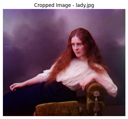
Assignment 1 : Colorizing the Prokudin-Gorskii Photo Collection
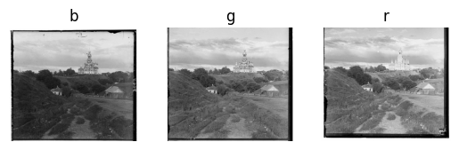
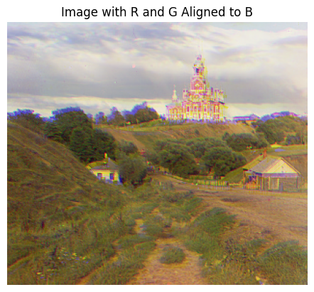
While using a window to align channels can be effective for low-resolution images,
this approach becomes impractical for higher-resolution images due to the increased computational cost.
Additionally, reducing the window size to mitigate computational demands risks missing the optimal alignment shift,
especially if the best shift falls outside the smaller window.
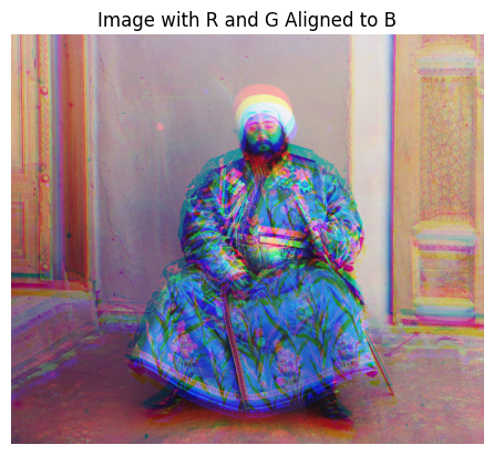
- emir.tif (3702 x 9627) : the alignment time: 141.69 seconds
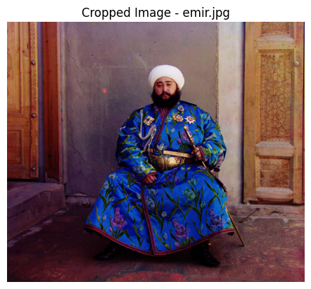
The significant difference in alignment time between the two images, "cathedral.jpg" and "emir.tif," primarily stems from the increase in computational complexity due to higher image resolutions. The single_scale_alignment function iterates over all possible shifts within a defined window, calculating the Sum of Squared Differences (SSD) for each shift. As the resolution of an image increases, the number of pixels to be processed grows, leading to an exponential increase in the number of calculations required. For the low-resolution image (cathedral.jpg), the computational cost is relatively low, resulting in a short alignment time of 0.44 seconds. However, for the high-resolution image (emir.tif), the vastly larger number of pixels significantly increases the computational burden, leading to a much longer alignment time of 141.69 seconds. Also as we can see in emir.tif image, there is the risk of missing the optimal alignment shift that could occur when using a small window on a high-resolution image directly. To address this issue, the concept of an image pyramid can be employed
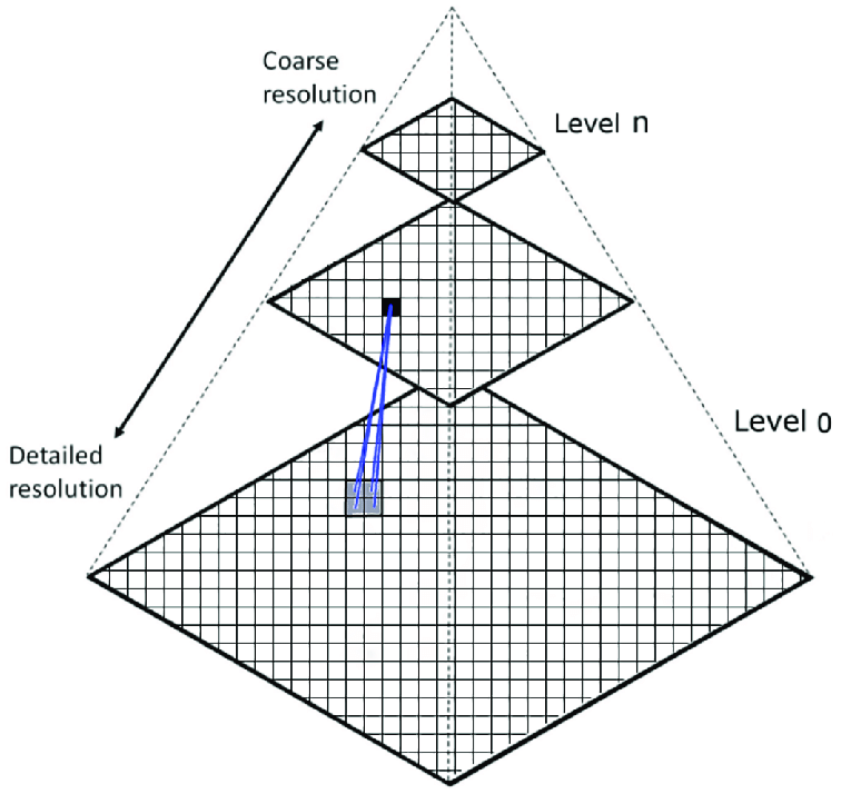
Multiscale alignment using image pyramids is a technique designed to efficiently align images through a hierarchical approach.
This process involves creating a series of images of decreasing resolutions, forming a pyramid where each level represents the image at a different scale.
The alignment is performed starting from the lowest resolution (the top of the pyramid) and progressively moving to the highest resolution (the base of the pyramid).
The process are as follows:
1. For each image to be aligned, generate an image pyramid.
This involves downsampling the original image multiple times to create a set of images at decreasing resolutions.
2. Start the alignment at the highest level of the pyramid (lowest resolution).
Since the images are smaller, the computational cost is reduced.
Align the images using methods like the single_scale_alignment,
but the process is much faster due to the reduced image size.
3. Once the images are aligned at a coarse level, move down the pyramid to a higher resolution.
Use the shifts parameters found at the previous level as the starting point and refine the alignment at this level.
This step is repeated until the original resolution is reached.
Through this method, the computational efficiency is greatly enhanced because initial alignments are performed on smaller versions of the images. This reduces the number of calculations required, speeding up the alignment process.
Also starting with a coarse alignment and progressively refining it allows for more accurate alignment.
This method reduces the likelihood of getting trapped in local minima,
which is a common issue when performing alignment at a single scale with a small search window.
Therefore the multiscale approach is more robust to noise and other artifacts. Initial alignments at lower resolutions are less affected by fine-scale noise, leading to a more stable alignment process.
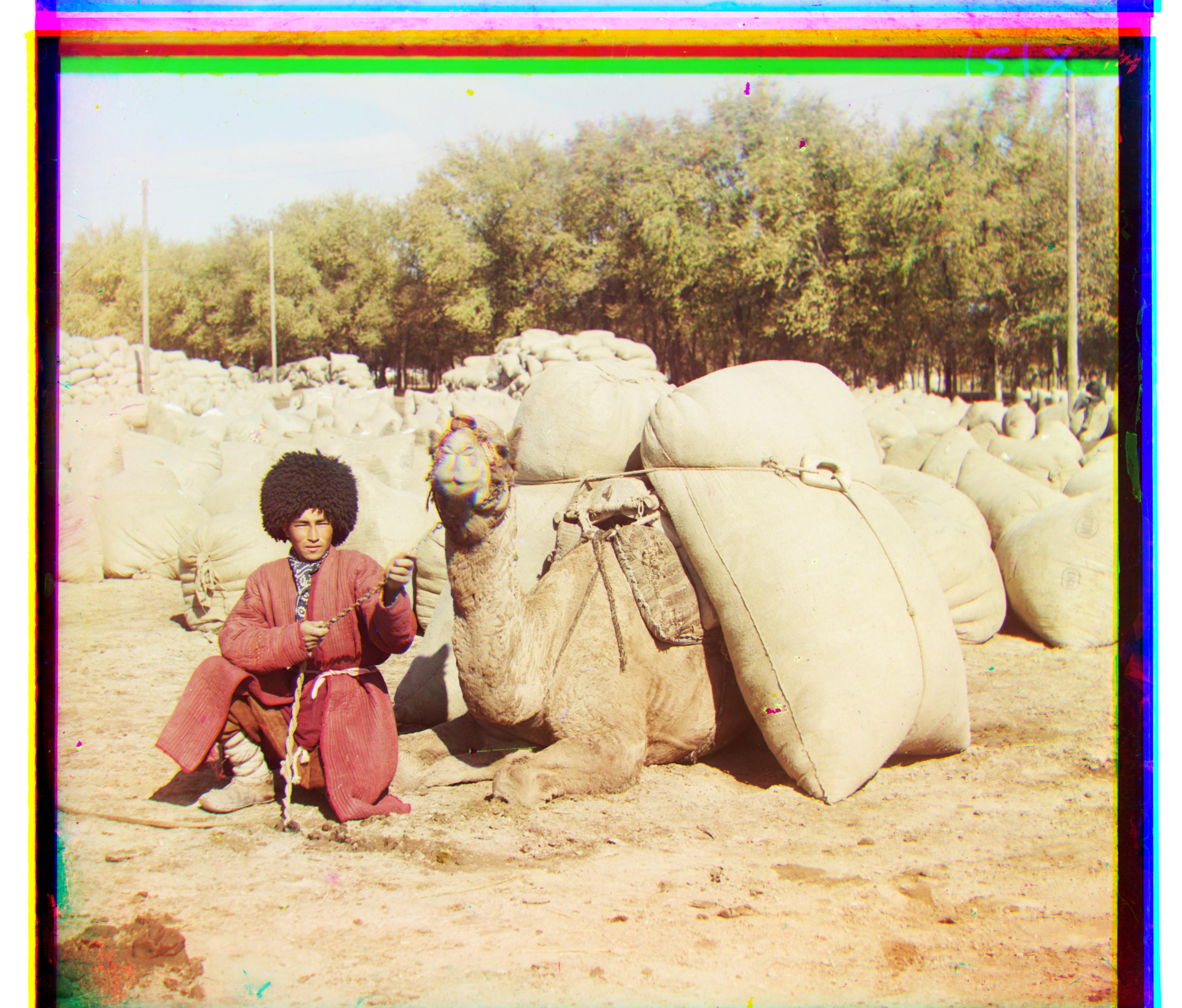
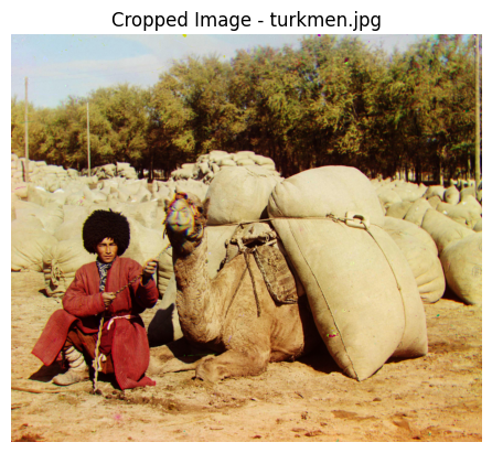
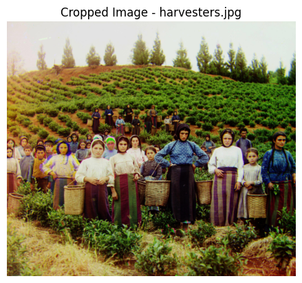
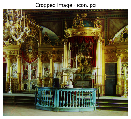
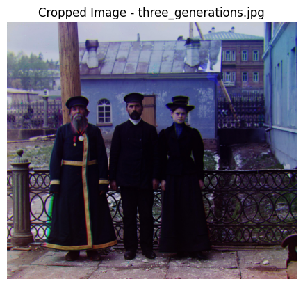
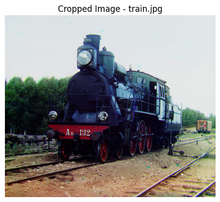
R translate(116, 28), G translate(56, 21)
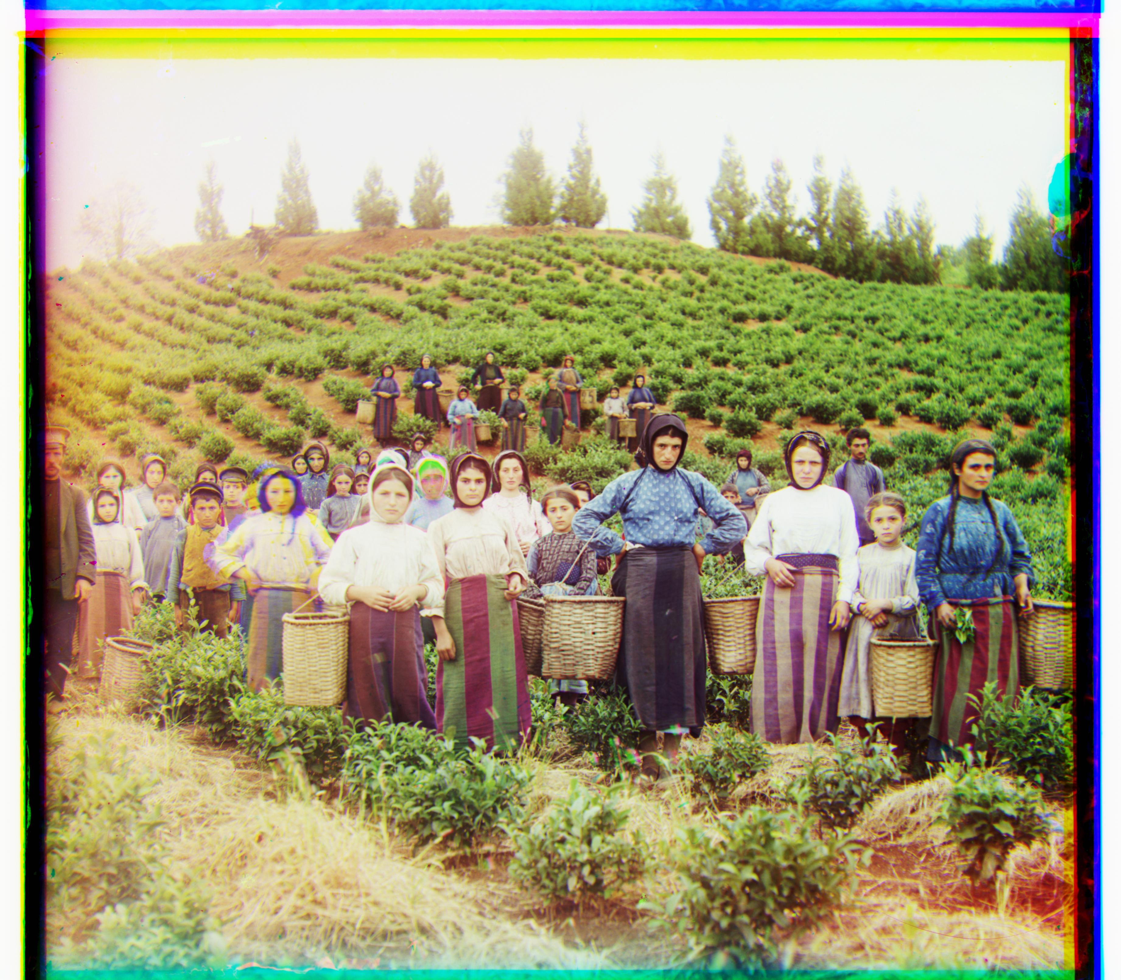
R translate(120, 11), G translate(52, 9)
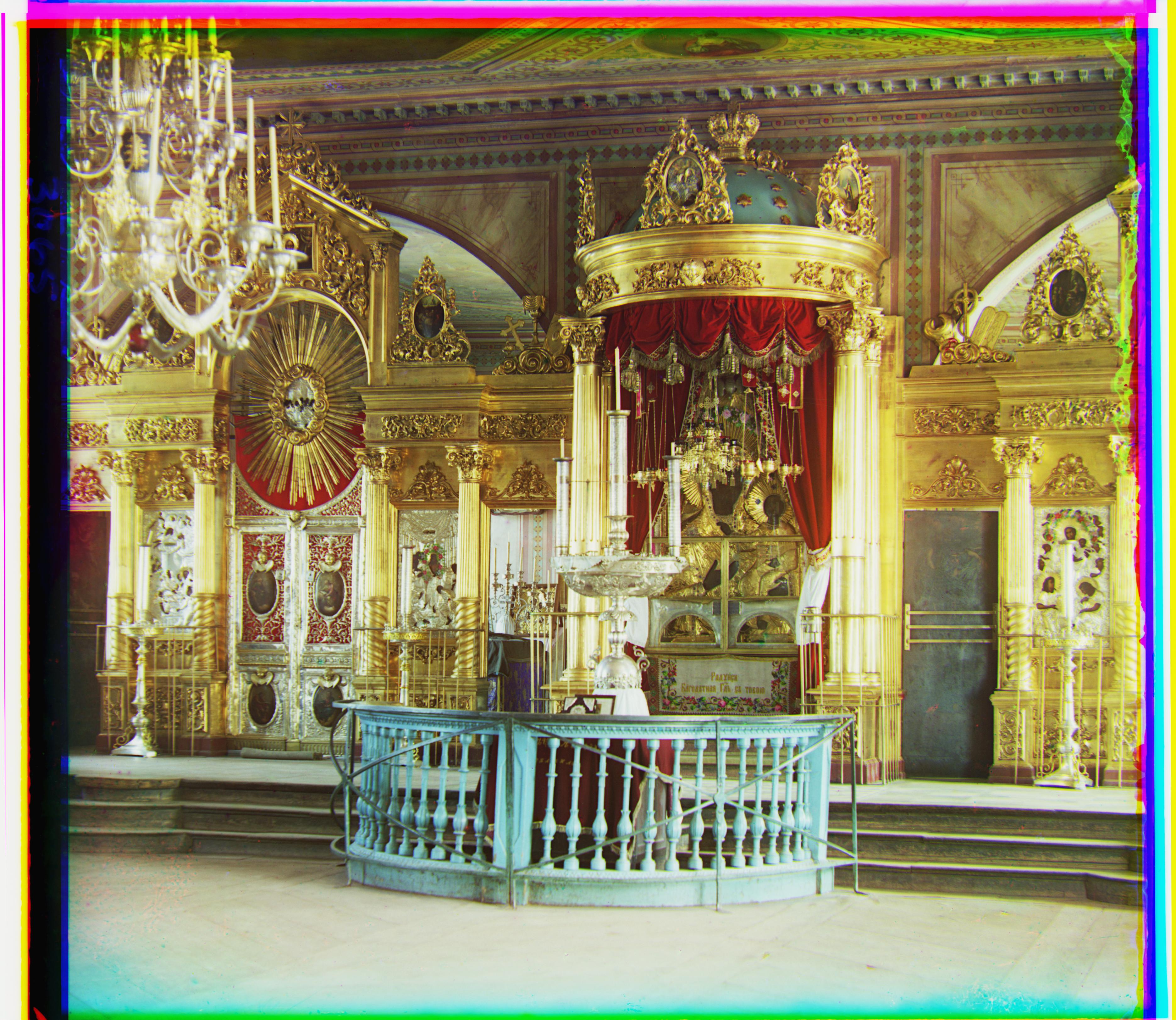
R translate(90, 23), G translate(41, 17)
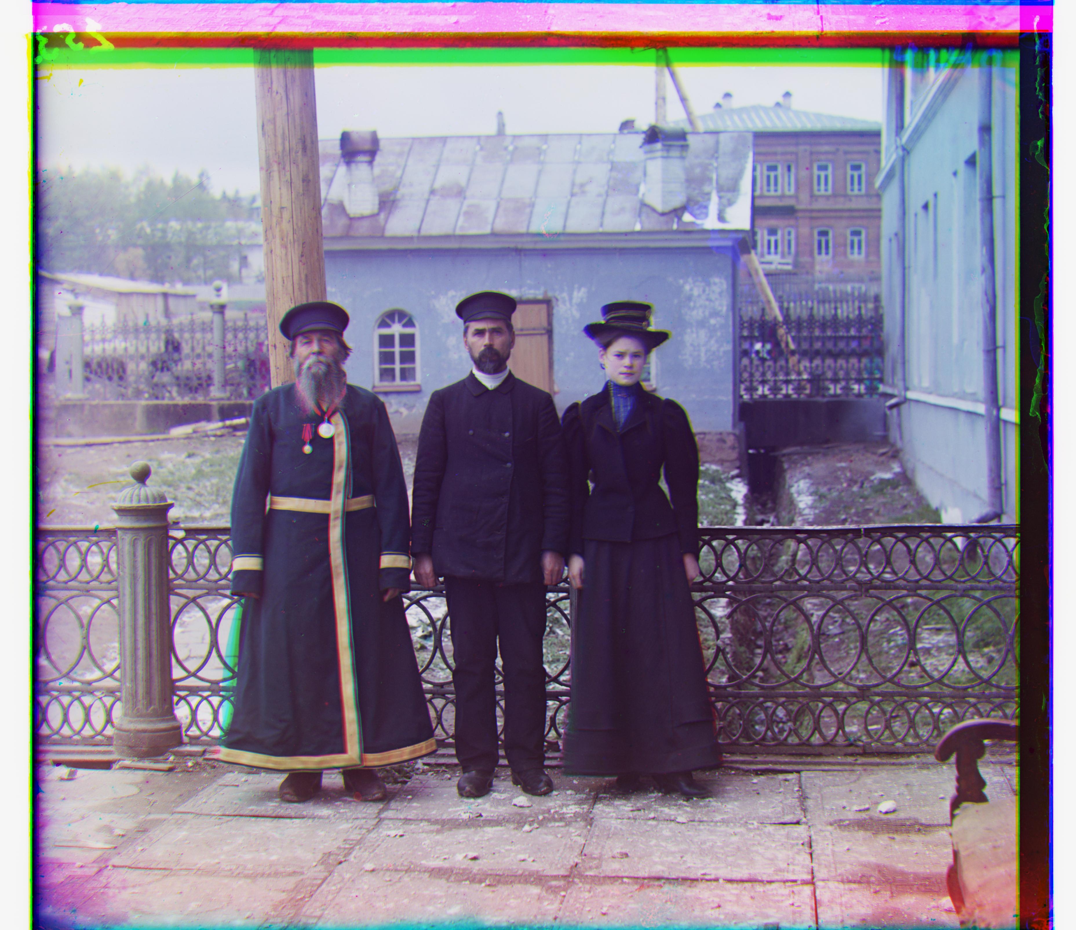
R translate(112, 11), G translate(53, 14)
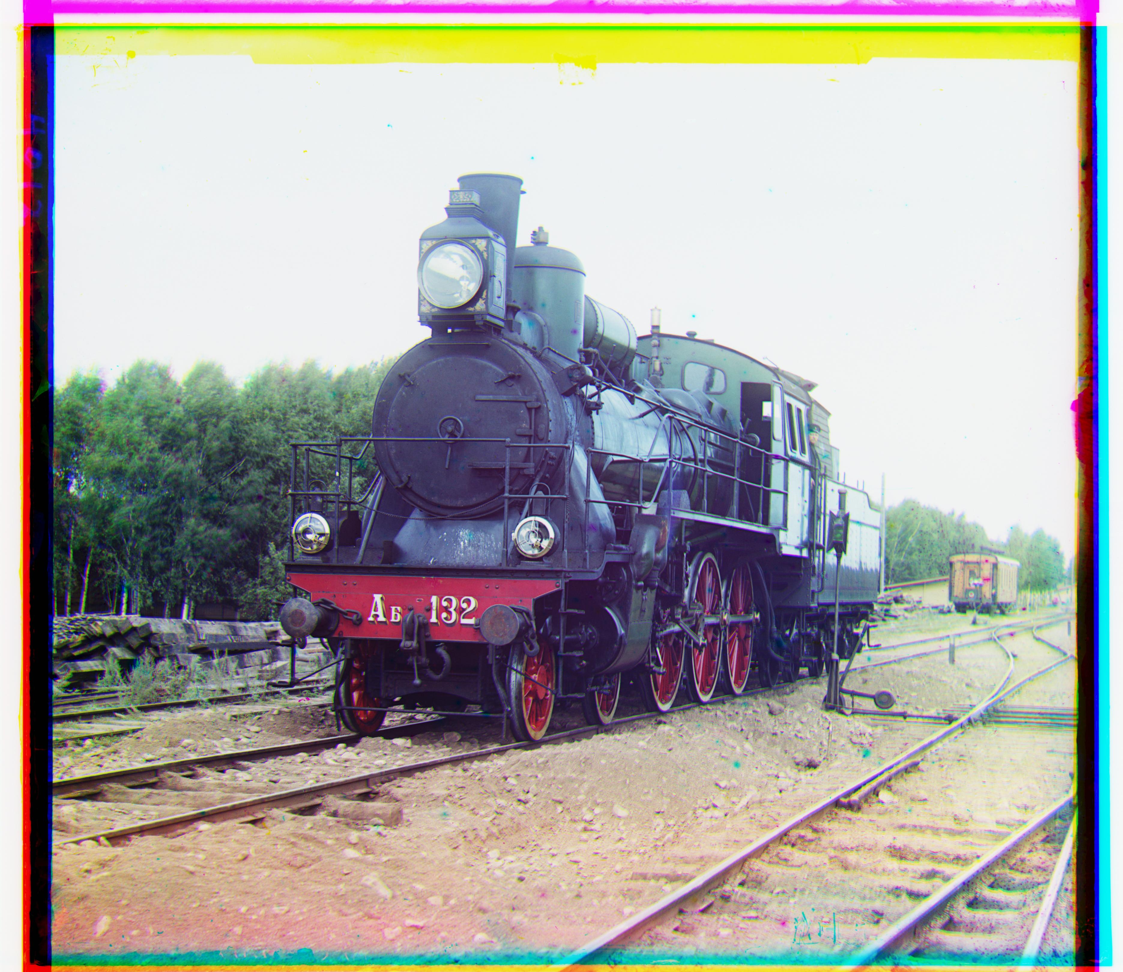
R translate(87, 32), G translate(42, 6)
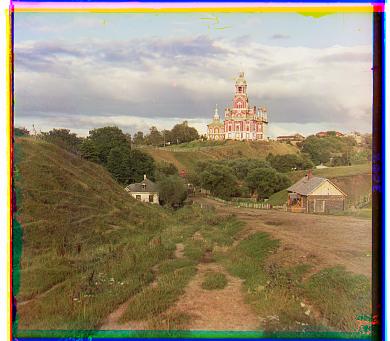
R translate(12, 3), G translate(5, 2)
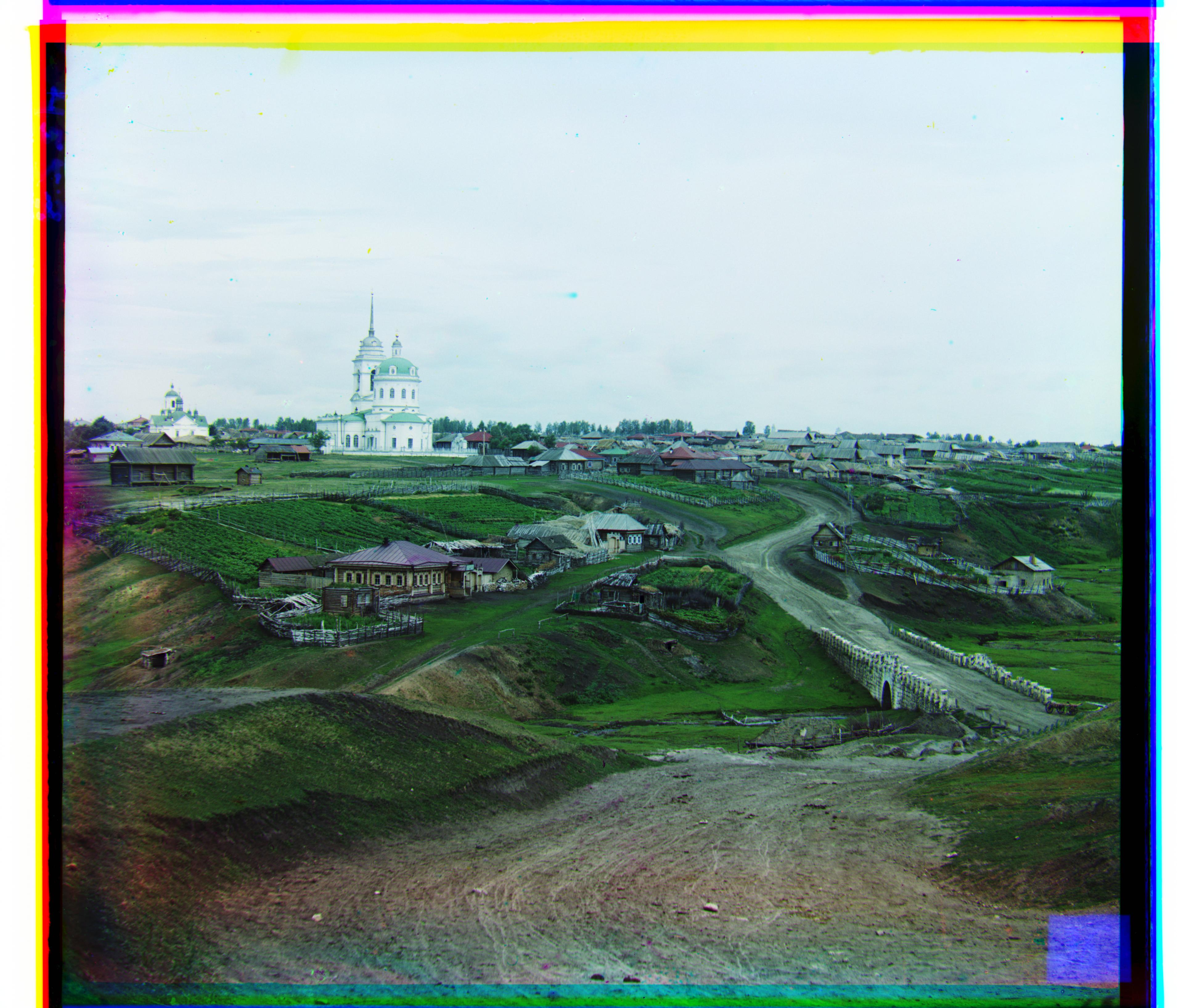
R translate(138, 22), G translate(64, 12)
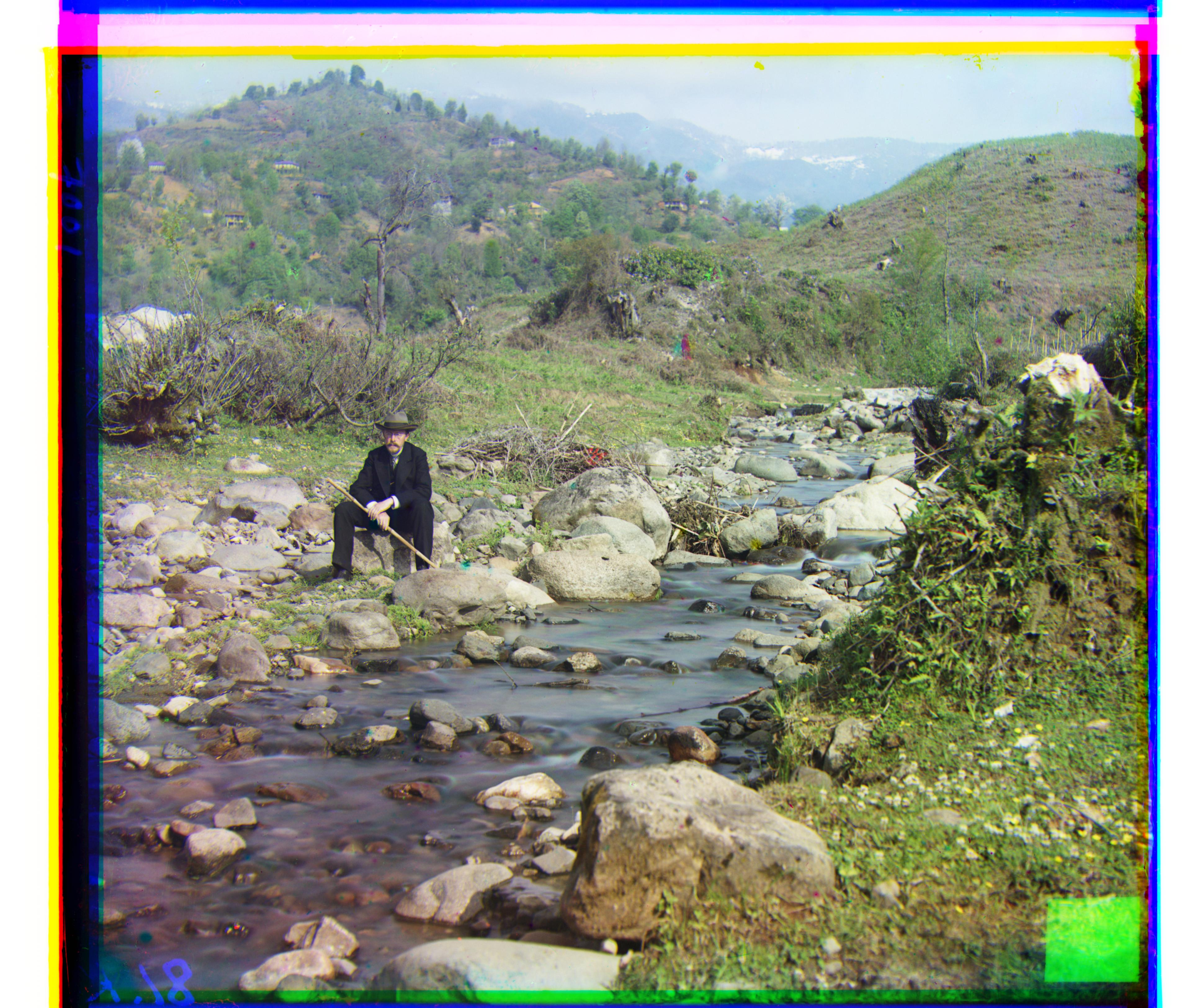
R translate(176, -3773), G translate(79, -3781)
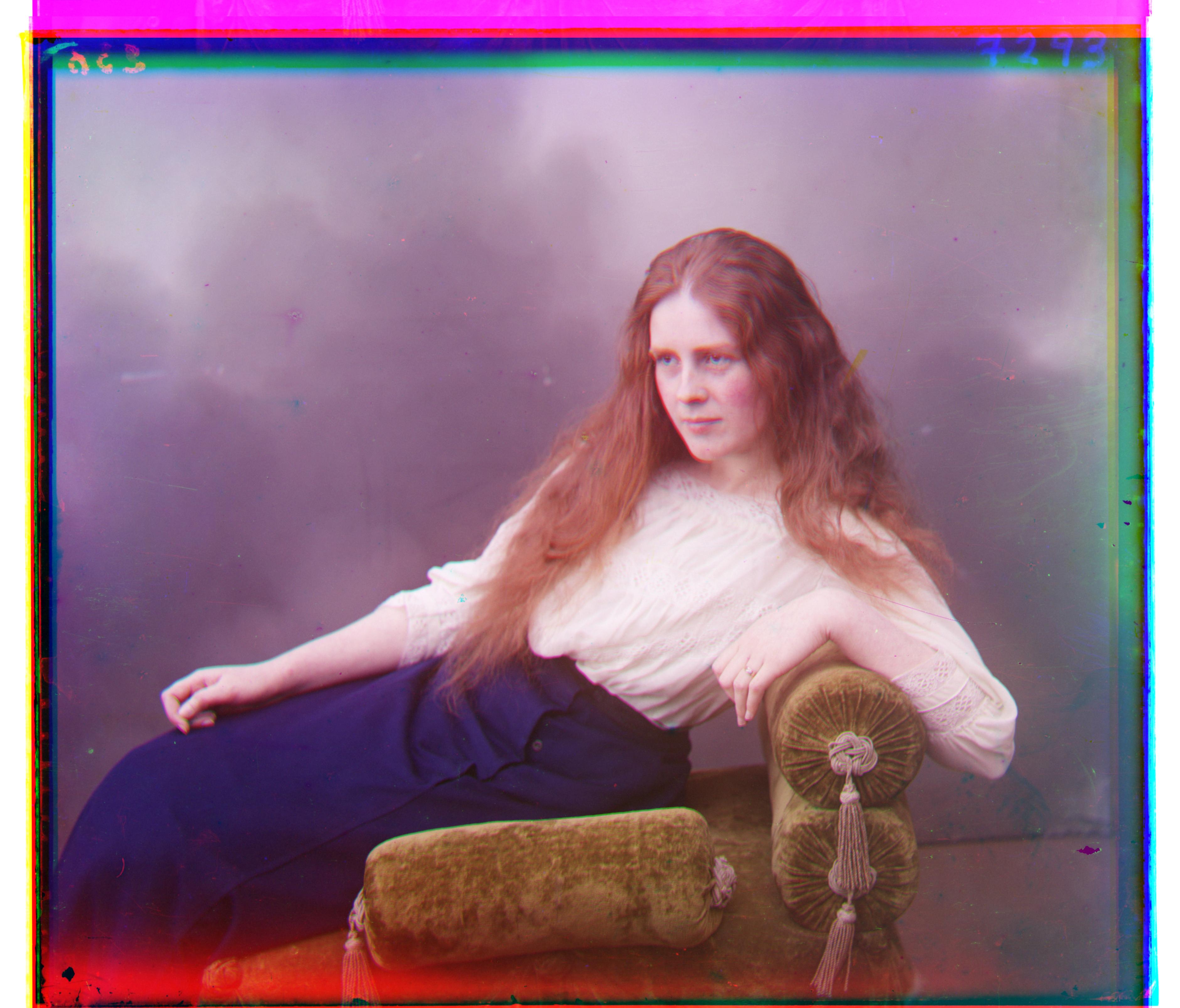
R translate(120, 11), G translate(52, 9)
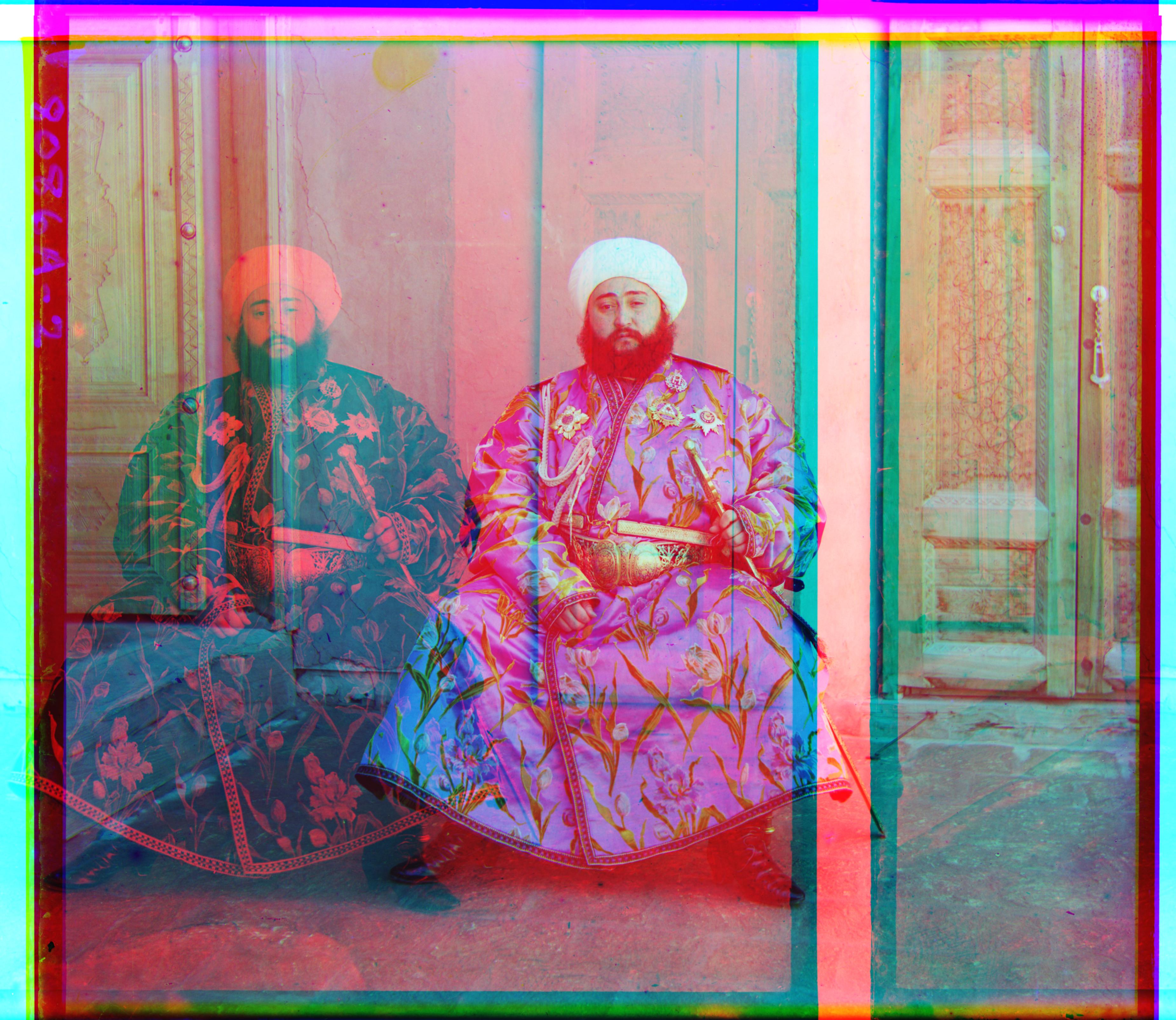
R translate(128, -1047), G translate(49, 24) - before histogram matching
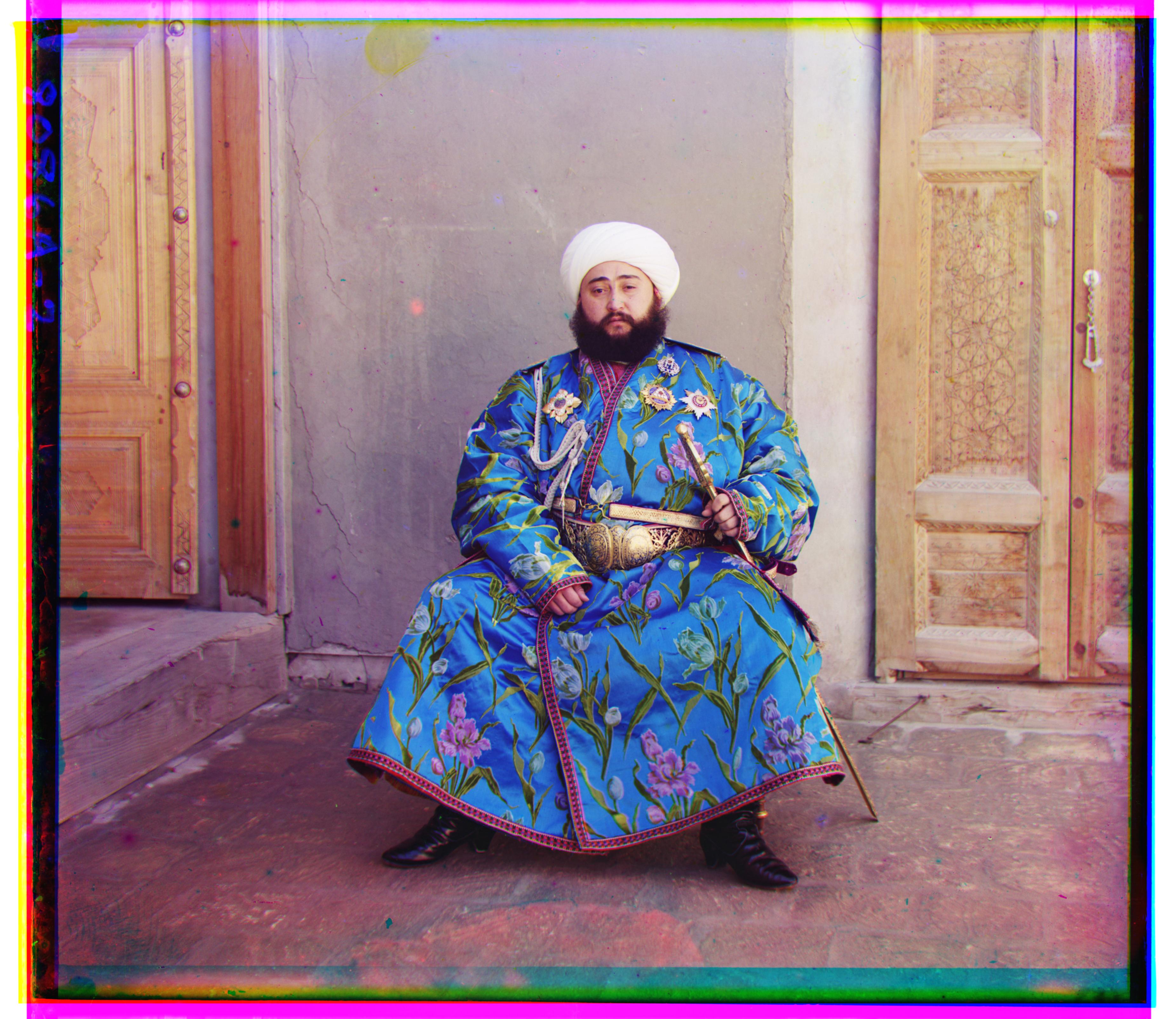
R translate(57, 17), G translate(-3, 7) - after histogram matching
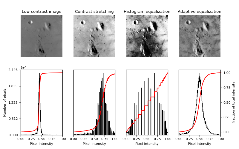
Auto contrast adjustment aims to improve the overall contrast of an image by redistributing the pixel intensities across the entire dynamic range.
This adjustment involves two main steps:
First, the algorithm computes the minimum and maximum intensity values present in the image.
These values represent the darkest and brightest pixels, respectively.
After determining the minimum and maximum intensity values, the algorithm linearly scales the pixel intensities so that the darkest pixel becomes black
(intensity value 0) and the brightest pixel becomes white (intensity value 1).
This normalization process stretches the intensity range, making darker regions darker and brighter regions brighter,
thereby enhancing the overall contrast of the image.
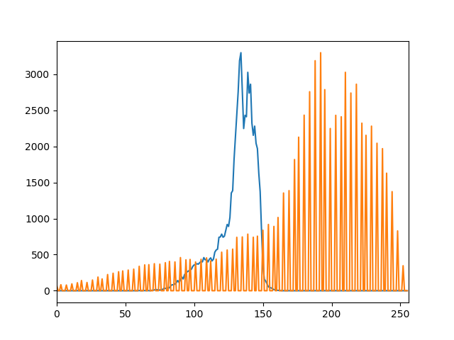
After twp steps, I added contrast enhancement process. Contrast enhancement involves further boosting the contrast of the image. This enhancement is achieved by applying a power-law transformation to the pixel intensities.
The algorithm scales the pixel intensities of the image to the range [0, 1], similar to the auto contrast adjustment step. This step ensures that the pixel values are within a manageable range for subsequent processing.
After scaling the pixel intensities, the algorithm applies a power-law transformation to the intensities. This transformation raises each pixel intensity to a specified power (commonly referred to as the contrast enhancement factor).
By adjusting the contrast enhancement factor, the algorithm can control the degree of contrast enhancement applied to the image.
Higher values of the contrast enhancement factor result in more pronounced differences between pixel intensities, leading to greater contrast enhancement.
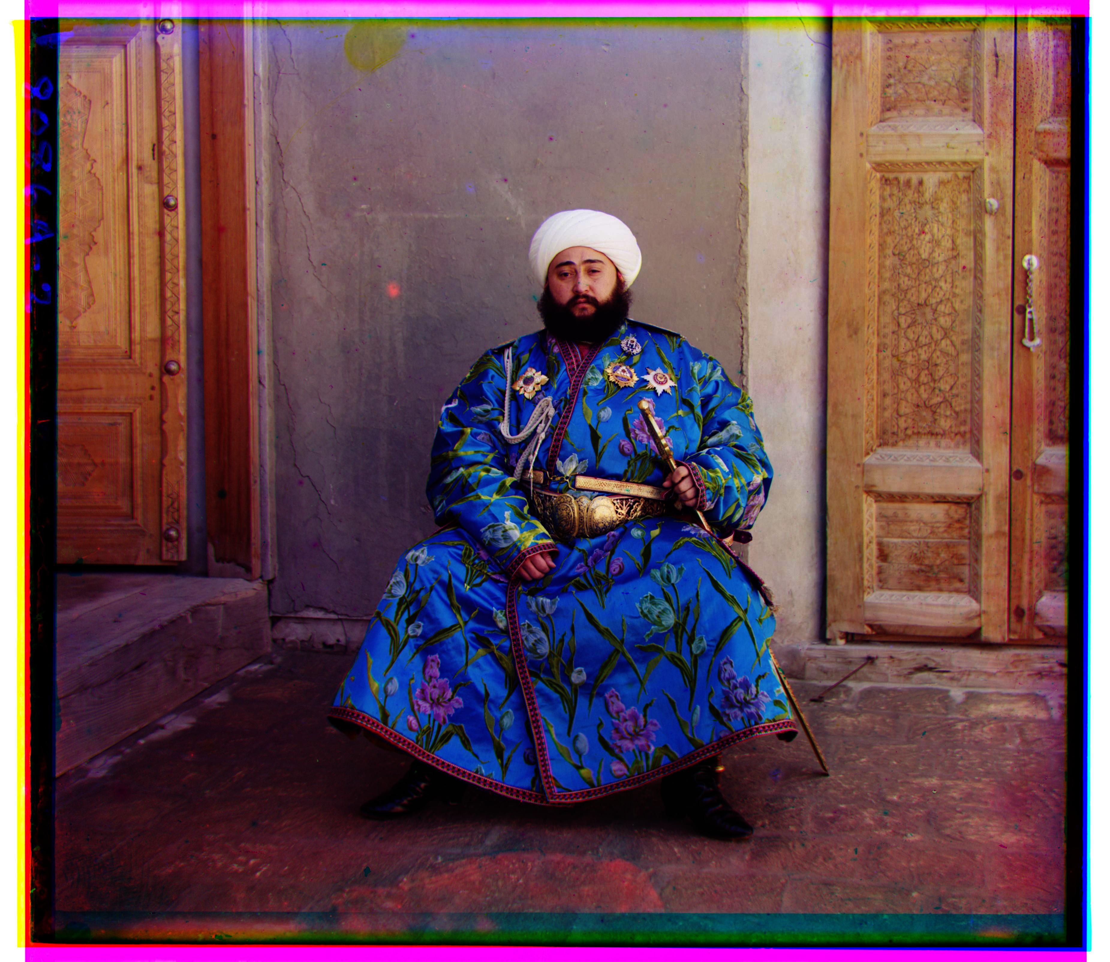
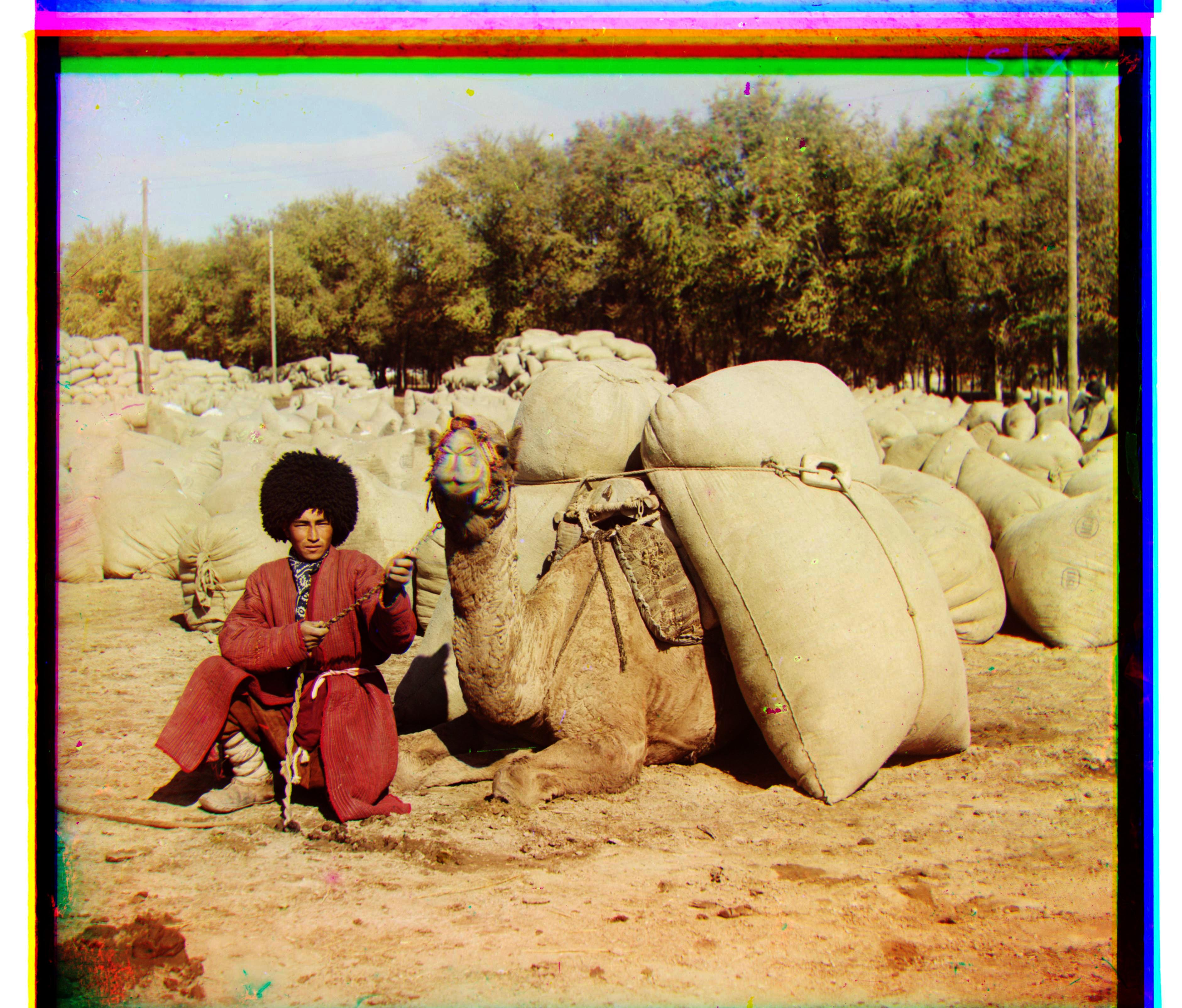
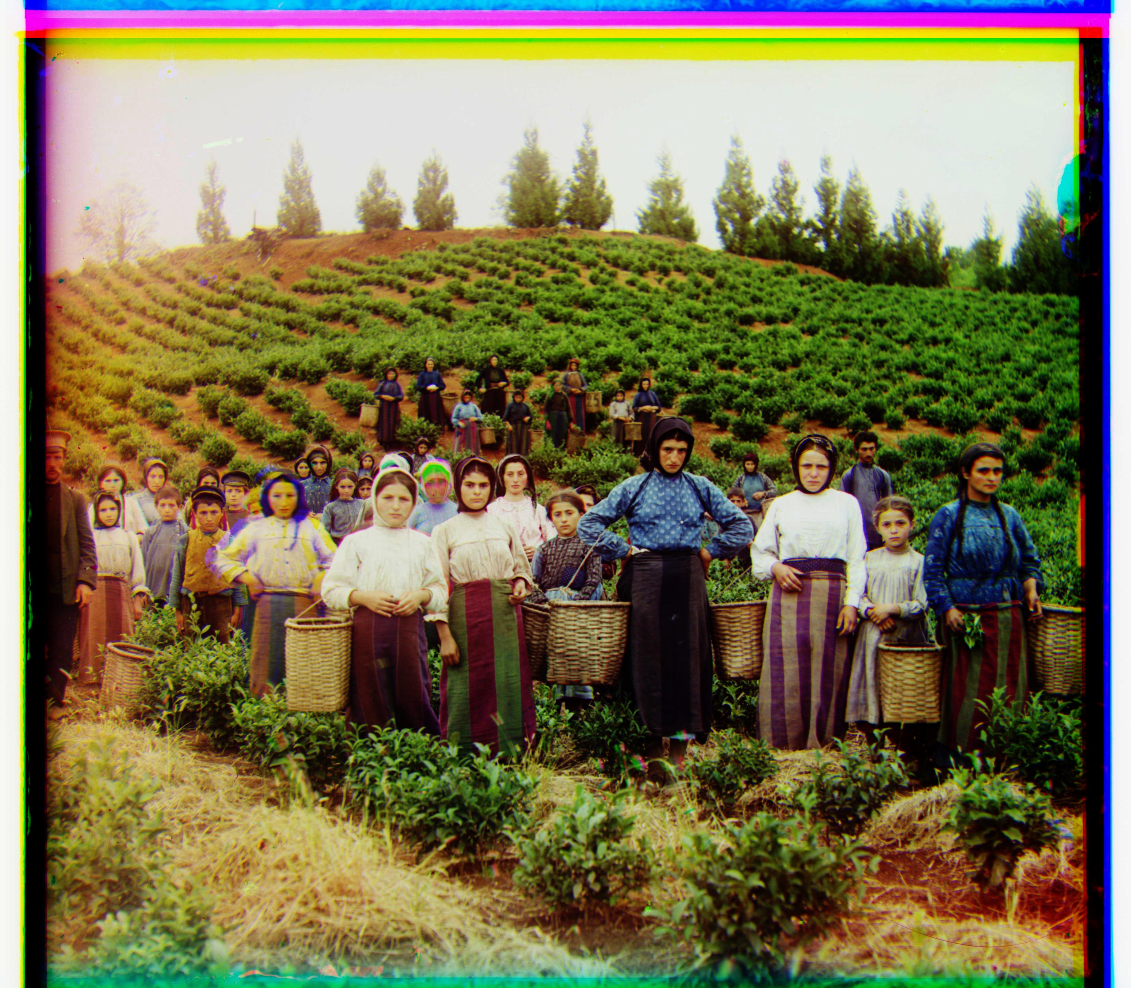
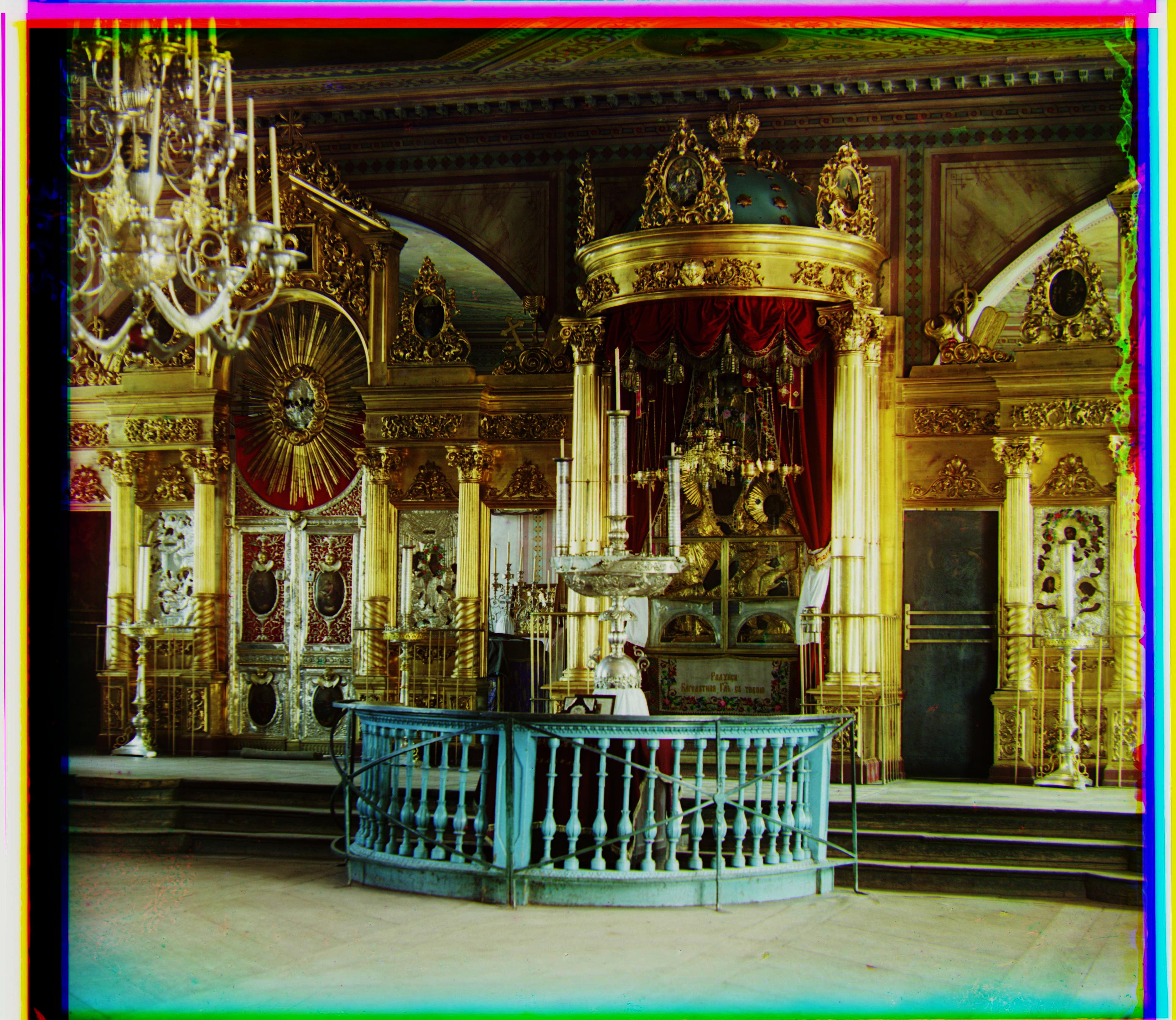
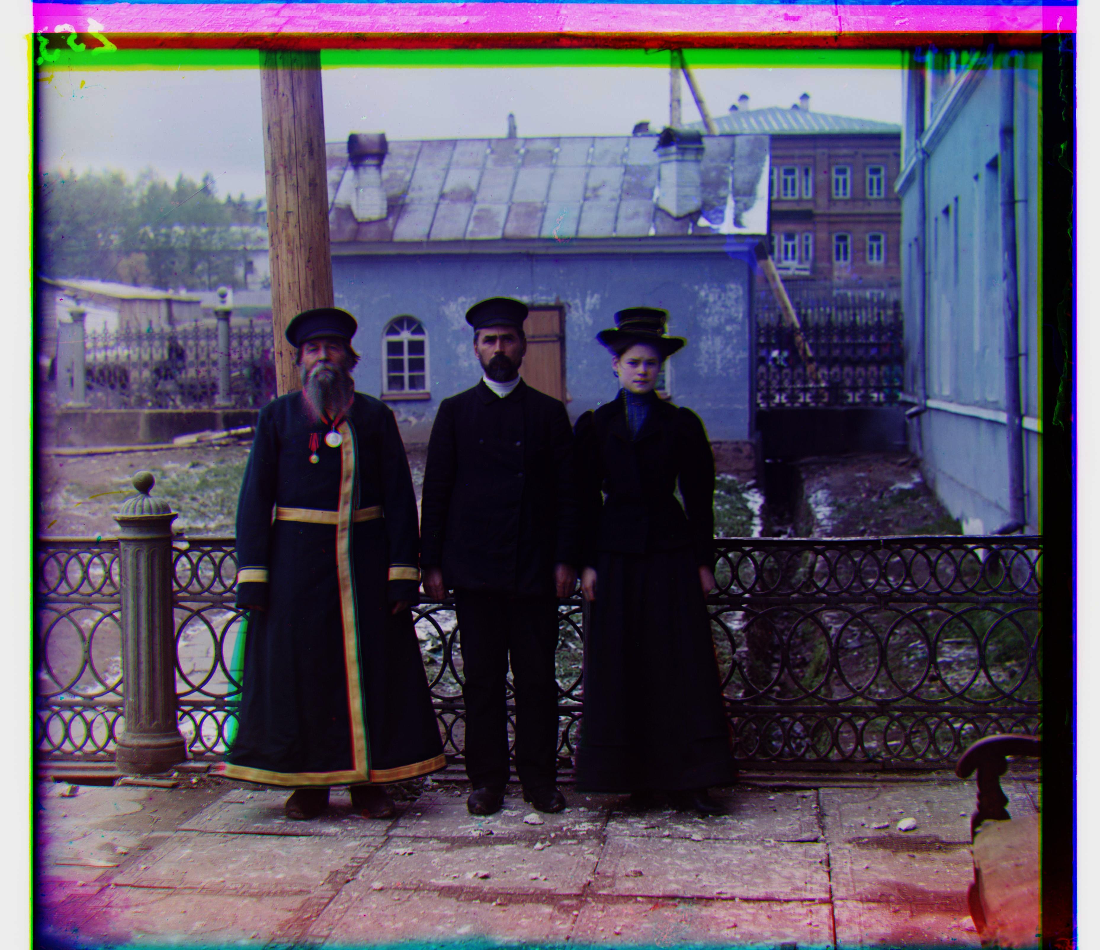
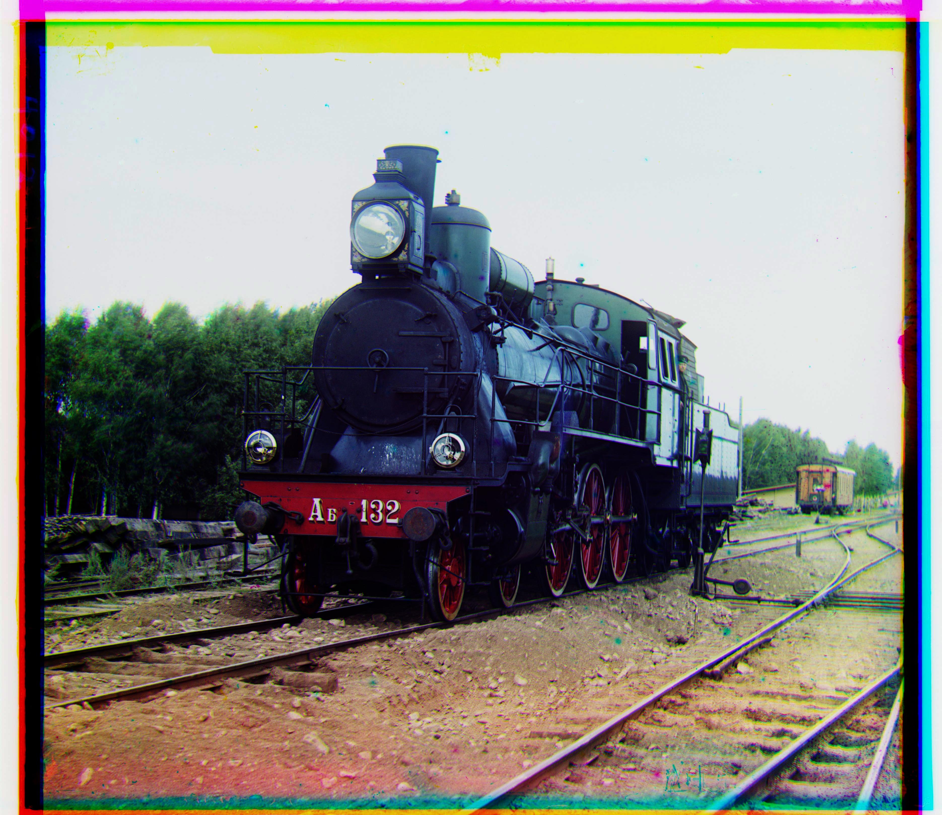
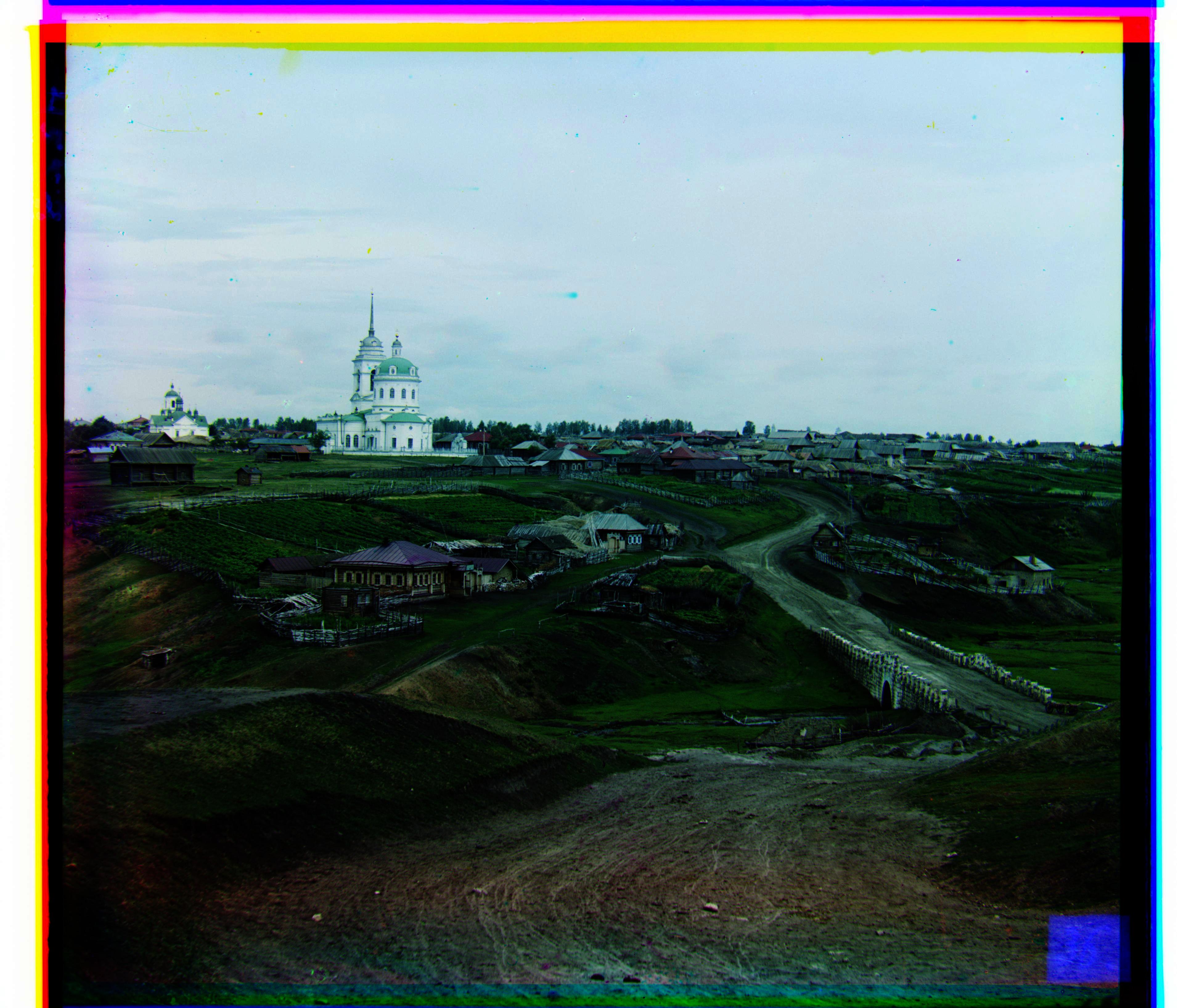
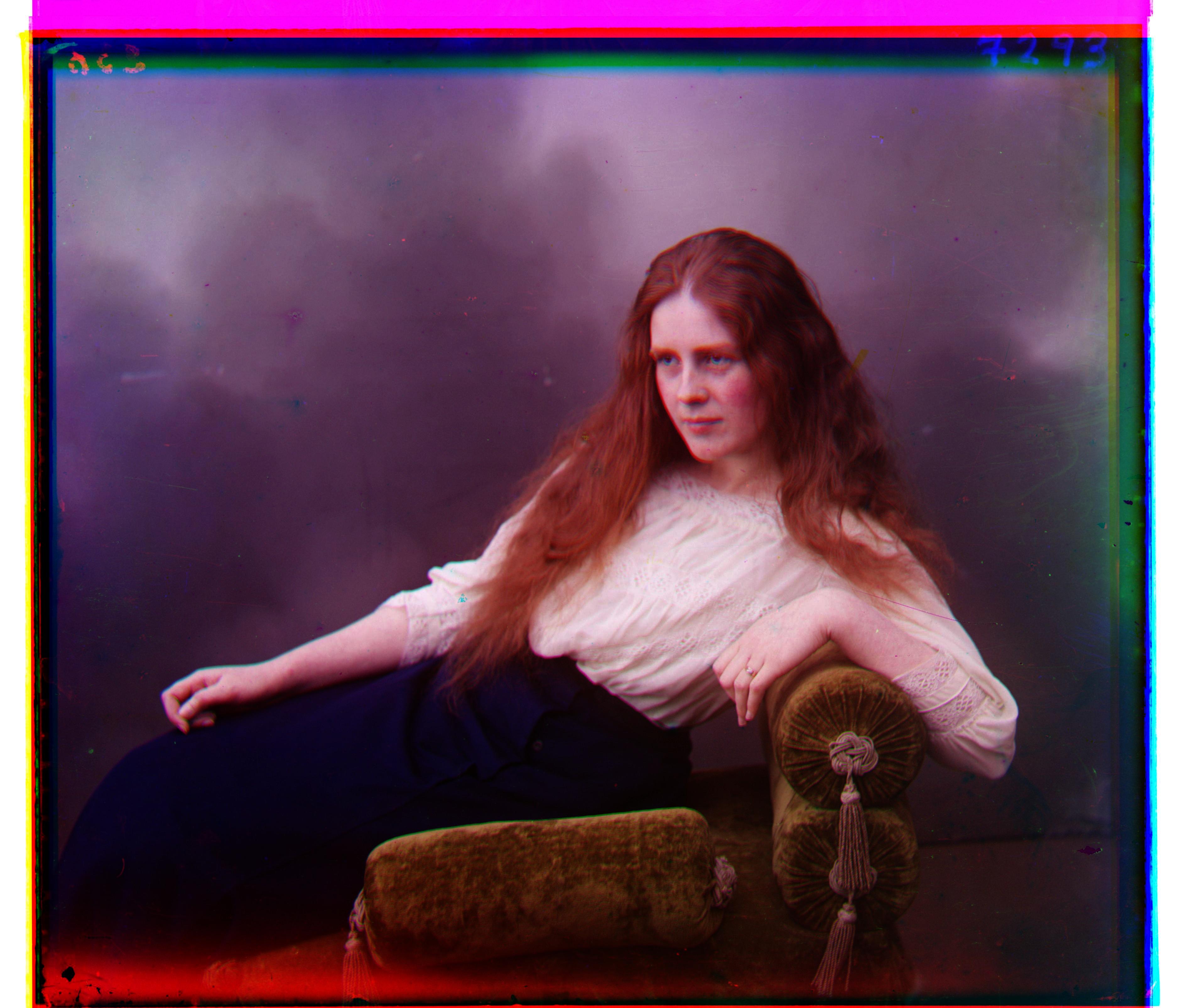
Auto Cropping has following steps. First, after preprocessing, the image is processed to highlight its edges.
This edge detection is a critical step for distinguishing between different shapes and lines that define the boundaries of objects within the image.
It simplifies the image to its basic structural components, making it easier to analyze geometrically.
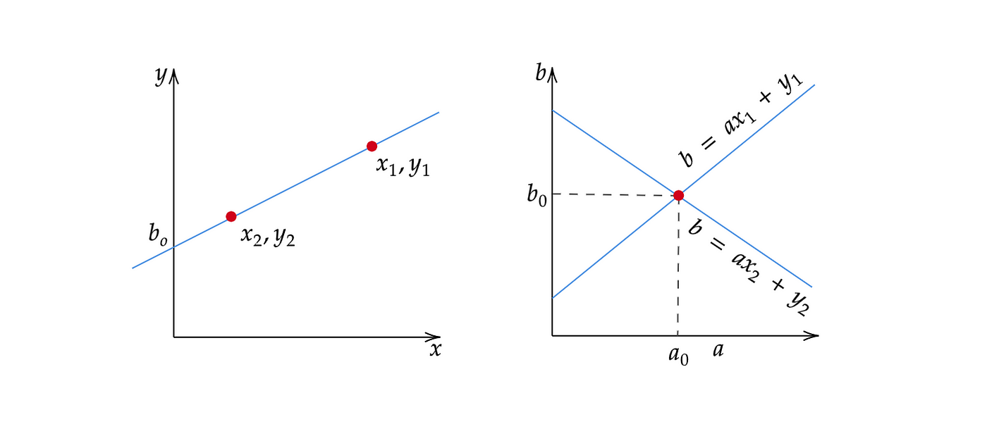
The core of line detection process involves using the Hough Transform, a technique for detecting lines within the image.
Unlike simple edge detection, the Hough Transform can identify and represent straight lines, even in noisy image data. As we can see the graph below, hough transform allows line detection by finding dot in hough transformed space.
In otherword, it works by mapping points from the image space to a parameter space and finding clusters of points that align along a line when plotted back in the image space.
This method is highly effective for recognizing the linear patterns that might outline objects or significant areas in the image,
making it indispensable for automated analysis.
After this process, by analyzing the positions of the lines detected by the Hough Transform,
the algorithm calculates the extremities of the area enclosed by these lines.
This involves finding the coordinates that define a bounding box around the area of interest,
essentially identifying the smallest rectangle that can contain all the detected lines.
With the boundaries clearly identified, the image is cropped to focus on the specific area enclosed by the detected lines.
This step significantly alters the image's dimensions to highlight the detected area, removing the parts of the original image that are outside these bounds.
Throughout this process, the code leverages the Hough Transform's capability to automate the detection of relevant lines and areas within an image.