Style Transfer
Experiments
Finetuning Content Loss
The content loss at a layer is defined as the MSE Loss between the features of the current image being optimized and the content image. Intuitively then it makes sense that the content loss would be most effective at conv_1 as this layer captures features that’re less abstract than downstream layers, less transformed, and closer to ‘true’ L2 pixel loss. This was my suspicion and it was confirmed. conv_1 loss converges much more quickly than loss at other layers. The following table shows the loss per layer per iteration.
| Name | 50 | 100 | 150 | 200 | 250 | 300 |
|---|---|---|---|---|---|---|
| Tubingen Conv1 | 0.000015 | 0.000008 | 0.000008 | 0.000008 | 0.000008 | 0.000008 |
| Tubingen Conv2 | 0.028442 | 0.002806 | 0.000591 | 0.000198 | 0.000068 | 0.000026 |
| Tubingen Conv3 | 0.230652 | 0.11514 | 0.078314 | 0.061757 | 0.054583 | 0.052213 |
| Tubingen Conv4 | 0.764896 | 0.338839 | 0.209798 | 0.149872 | 0.113488 | 0.089226 |
| Tubingen Conv5 | 2.271208 | 1.021523 | 0.680126 | 0.522512 | 0.432447 | N/A |
| Falling Water Conv1 | 0.000014 | 0.000003 | 0.000003 | 0.000003 | 0.000003 | 0.000003 |
| Falling Water Conv5 | 3.769431 | 2.087776 | 1.508189 | 1.20674 | 1.023051 | 0.896233 |
As you can see loss for conv_1 converges within the first 100 iterations and results in a lower overall loss than all the other layers. The loss for deeper layers is higher as expected. Throughout the rest of the experiments we’ll use conv_1 for our content loss.
Results of Finetuning Content Loss
| Noise Type | 0 | 50 | 100 | 150 | 200 | 250 | 300 |
|---|---|---|---|---|---|---|---|
| Noise 1 | 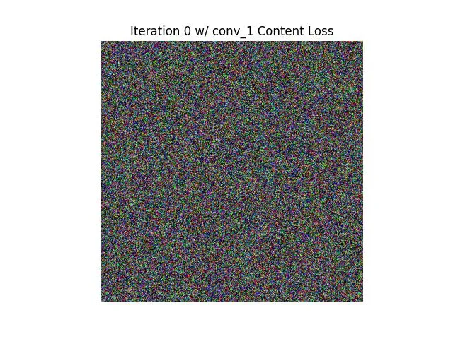 | 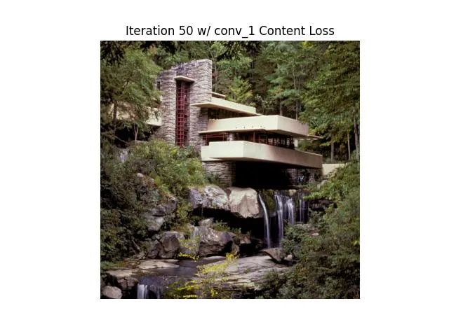 | 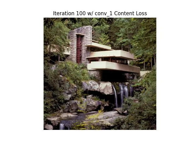 | 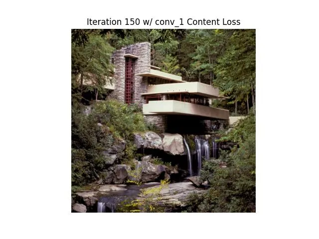 | 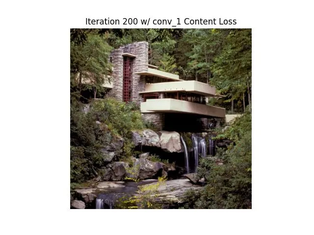 | 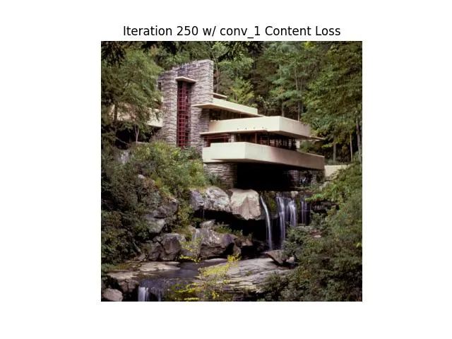 | 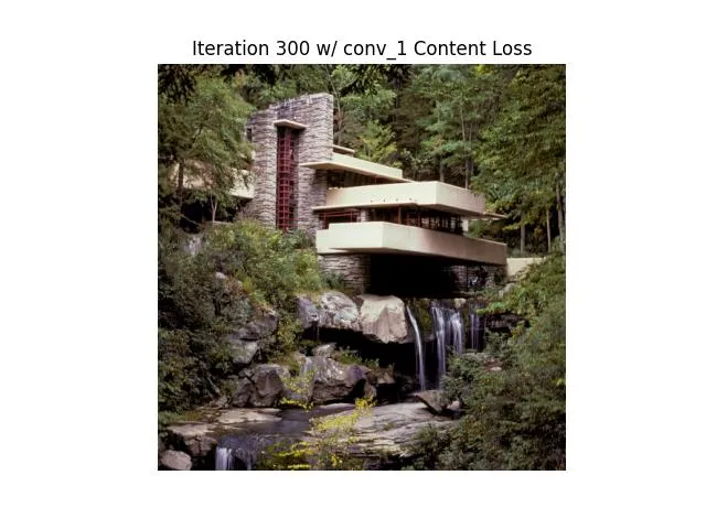 |
| Noise 2 | 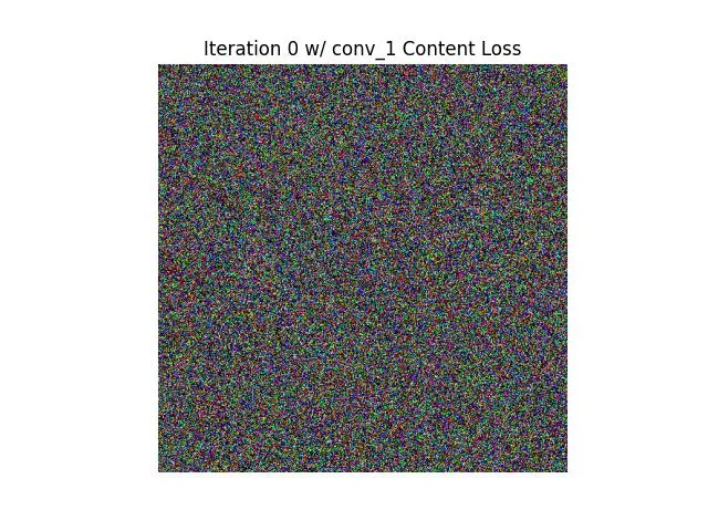 | 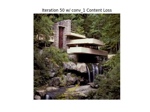 | 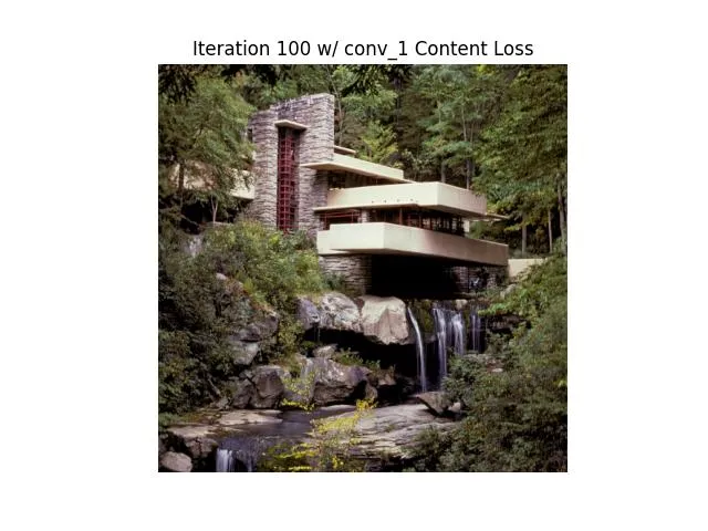 | 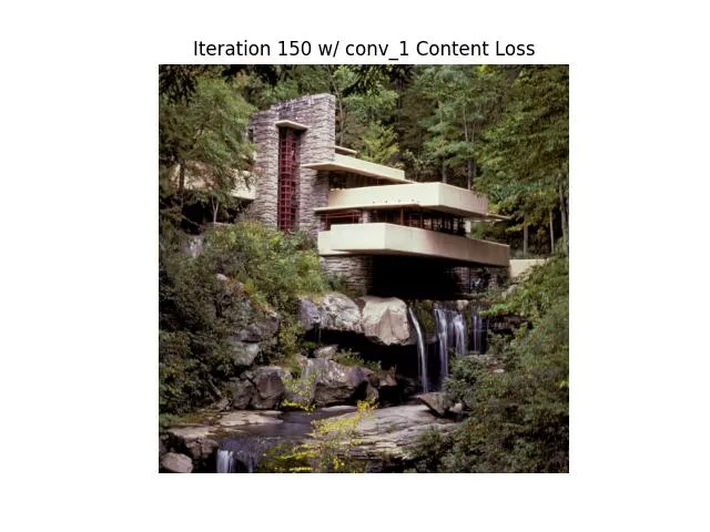 | 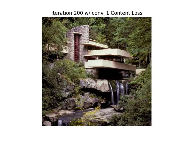 | 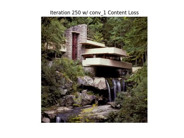 | 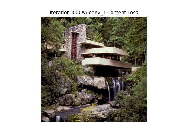 |
Here is a table of loss.
| Name | 50 | 100 | 150 | 200 | 250 | 300 |
|---|---|---|---|---|---|---|
| Noise 1 | 0.000014 | 0.000003 | 0.000003 | 0.000003 | 0.000003 | 0.000003 |
| Noise 2 | 0.000016 | 0.000002 | 0.000002 | 0.000002 | 0.000002 | 0.000002 |
The difference between the inputs was 1253 which makes sense as it’s just noise while their difference at the end was 3.41. Noise 1 had an L2 Loss of 2.5185 with ground truth while Noise 2 had an L2 Loss of 2.3263. Pretty good!
Texture Synthesis
Similar to content_loss we want to compute style loss as well. What is style loss? One idea is to use the Gram Matrix which is the correlation of two vectors in every dimension. This is just . We then want to minimize the loss between our computed gram matrix and the gram matrix encoding the style of our style target. Unlike content where as we get deeper the L2 loss becomes less meaningful with style it’s certaintly possible for important style information to be encoded by deeper layers.
To find the ideal style loss I just ran texture synthesis over all possible combinations of layers to calculate style loss at. The below table summarizes the results.
Texture Synthesis Tuning
Note the leftmost column indicates which conv layers were being used ie 12 --> conv_1, conv_2
| Conv Style Layers / Iteration Count | 0 | 50 | 100 | 150 | 250 | 300 |
|---|---|---|---|---|---|---|
| 1 | 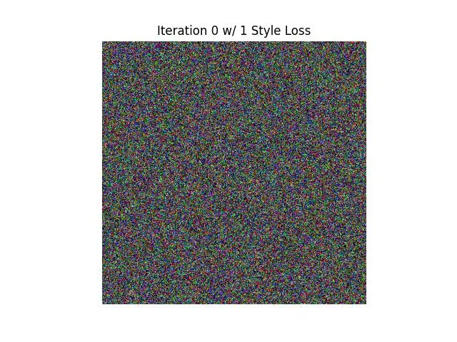 | 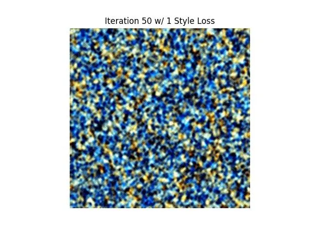 | 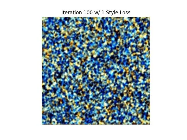 | 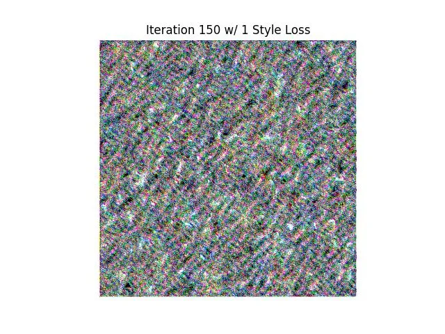 | 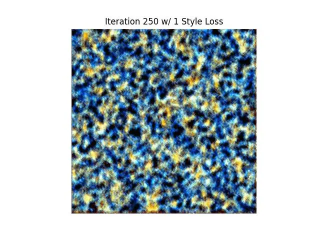 | 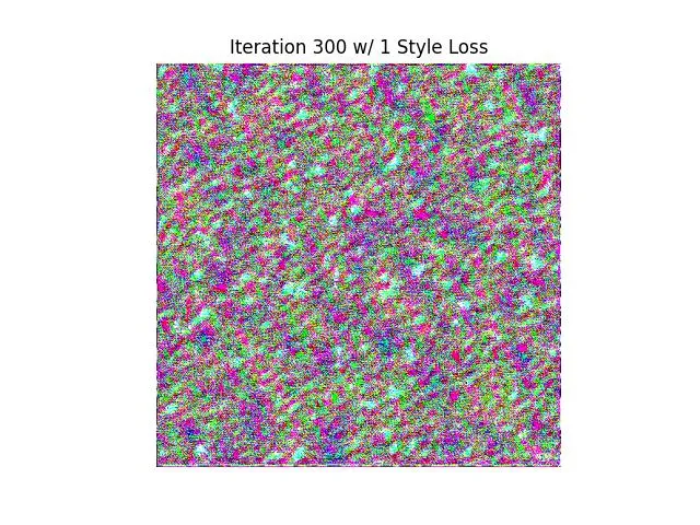 |
| 12 | 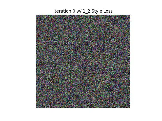 | 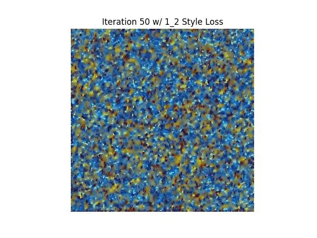 | 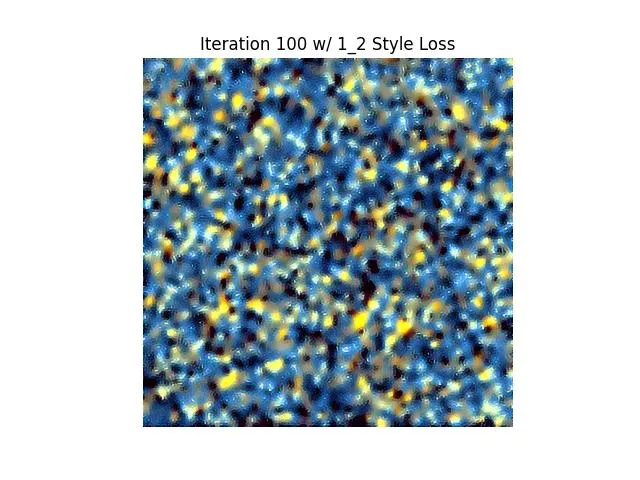 | 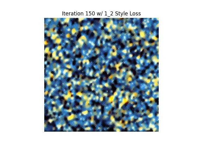 | 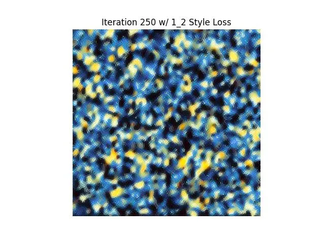 | 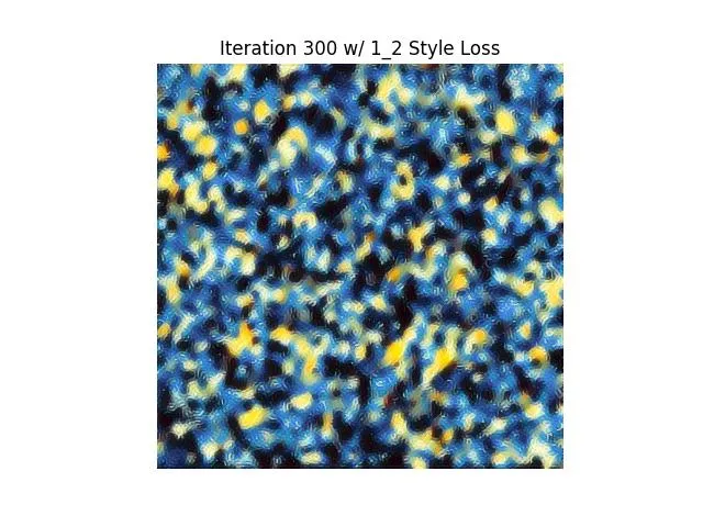 |
| 123 |  | 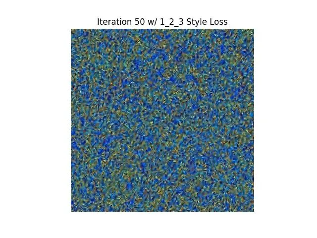 | 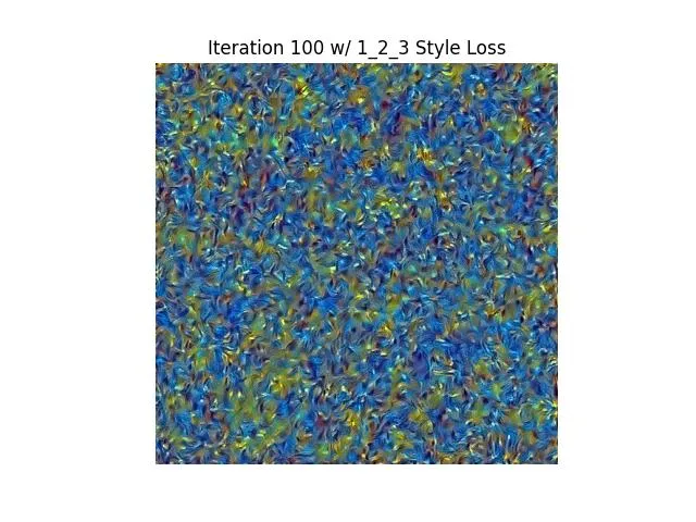 | 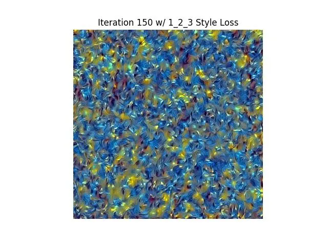 | 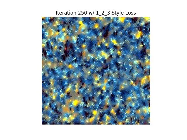 | 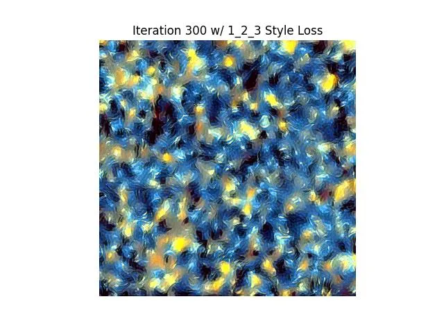 |
| 1234 | 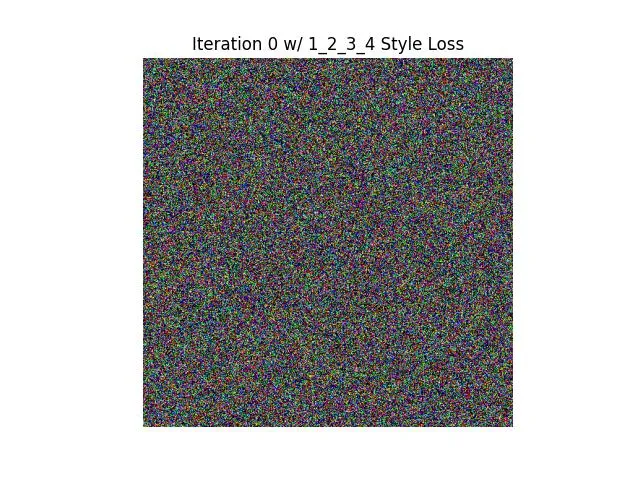 | 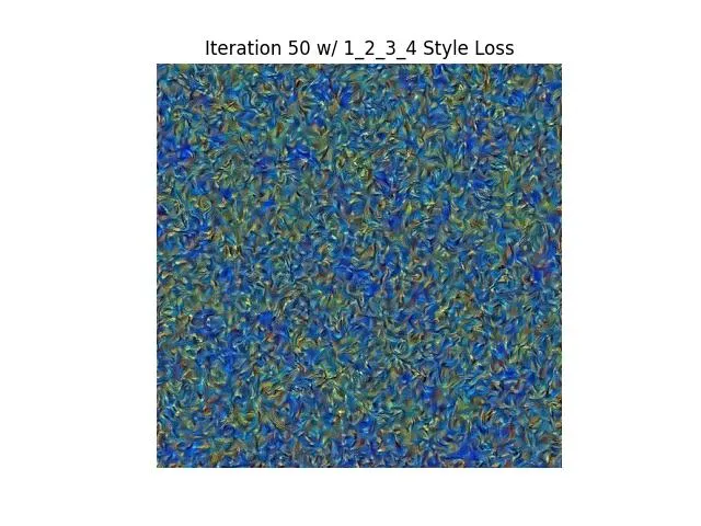 | 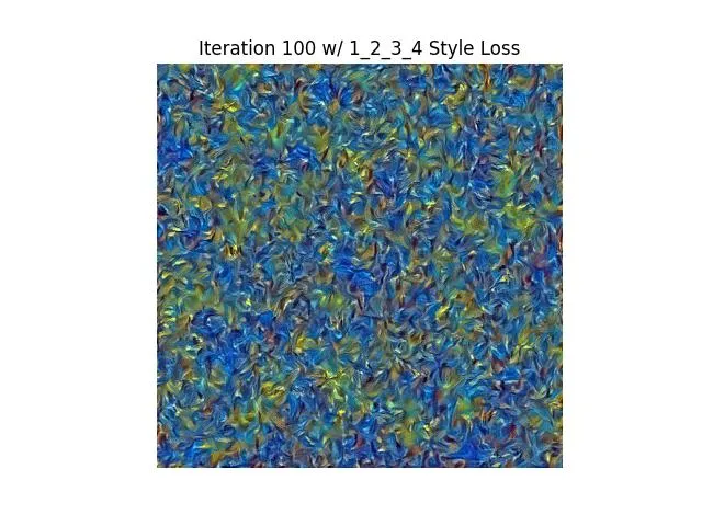 | 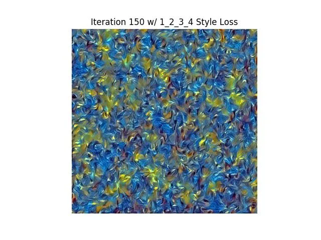 | 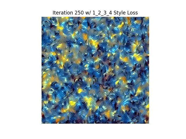 | 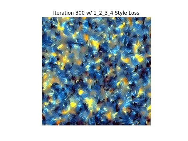 |
| 12345 | 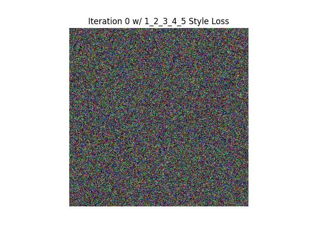 |  | 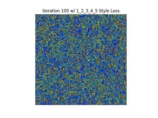 | 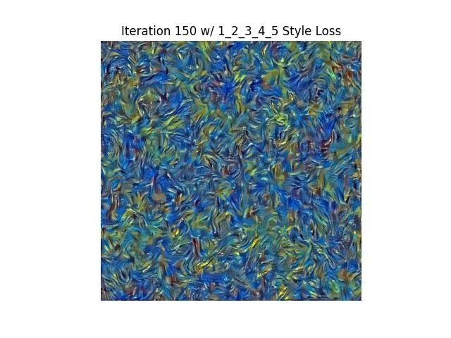 |  | 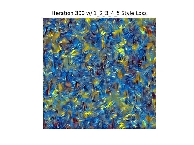 |
| 1235 |  | 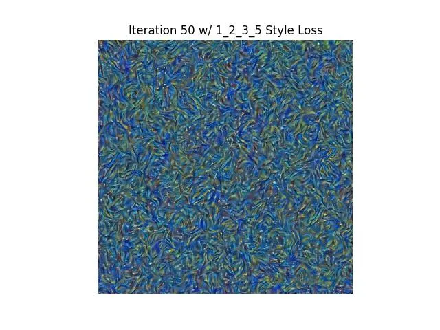 | 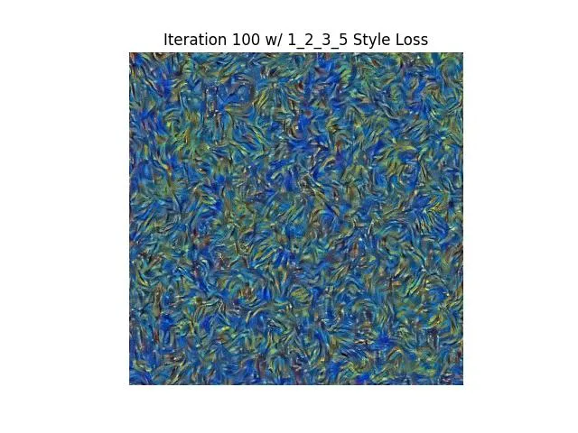 | 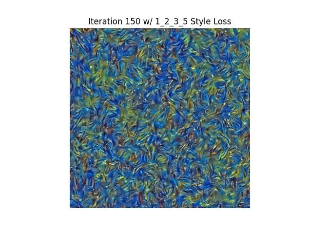 | 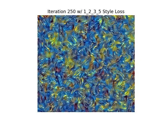 | 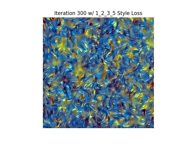 |
| 124 | 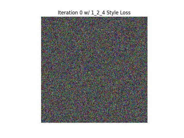 | 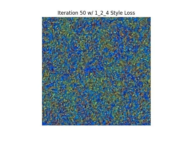 | 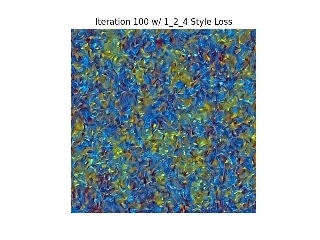 | 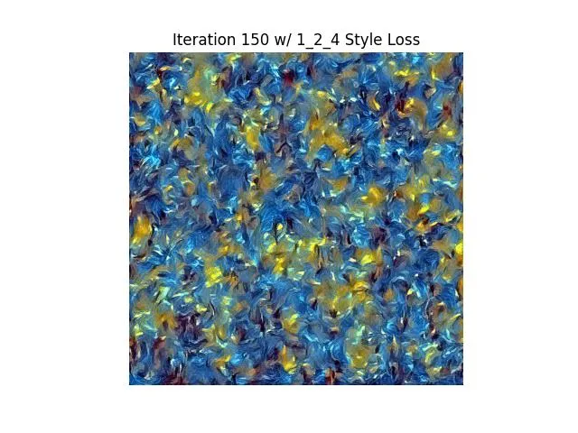 | 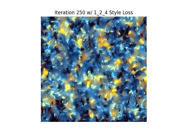 | 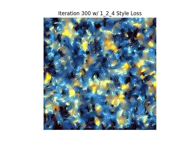 |
| 1245 | 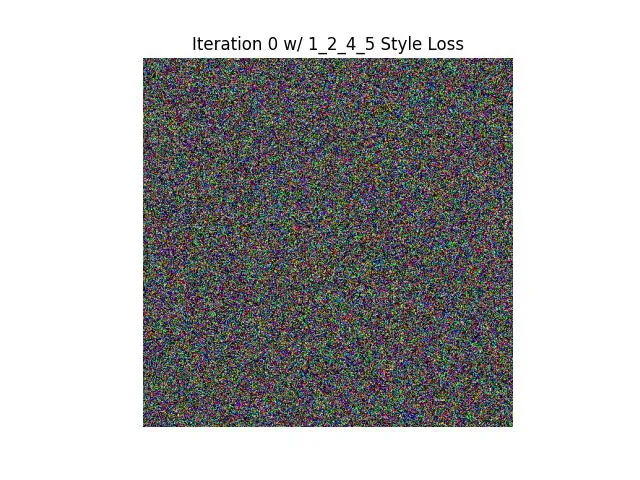 | 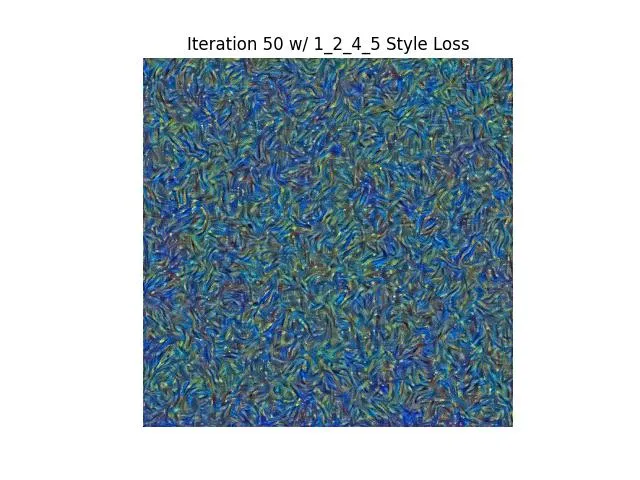 | 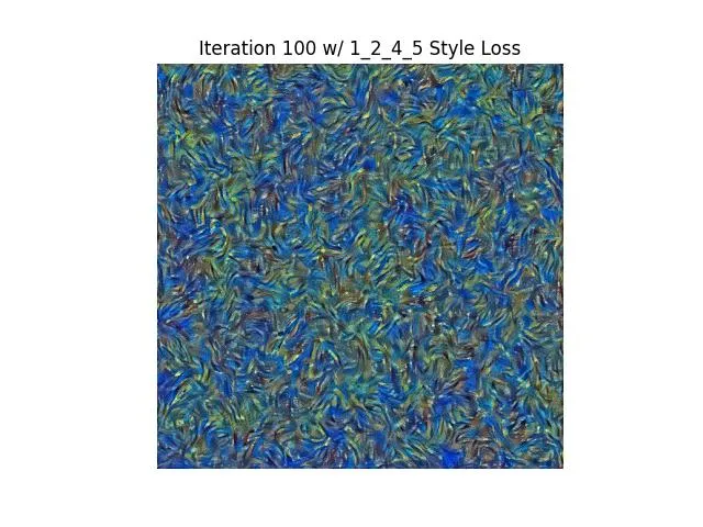 | 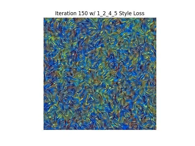 | 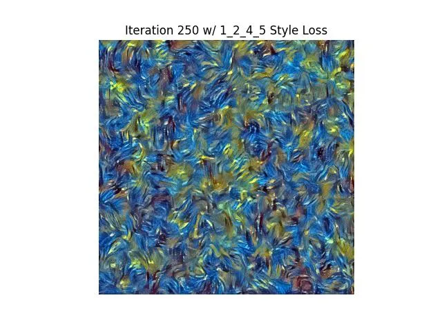 | 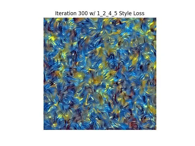 |
| 125 | 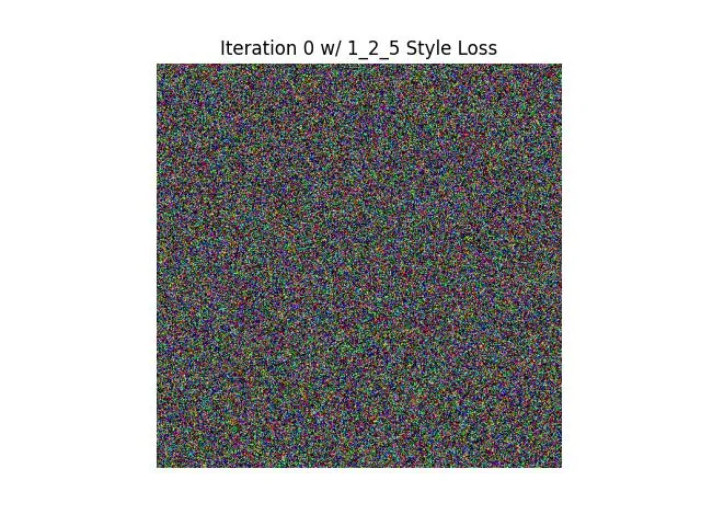 | 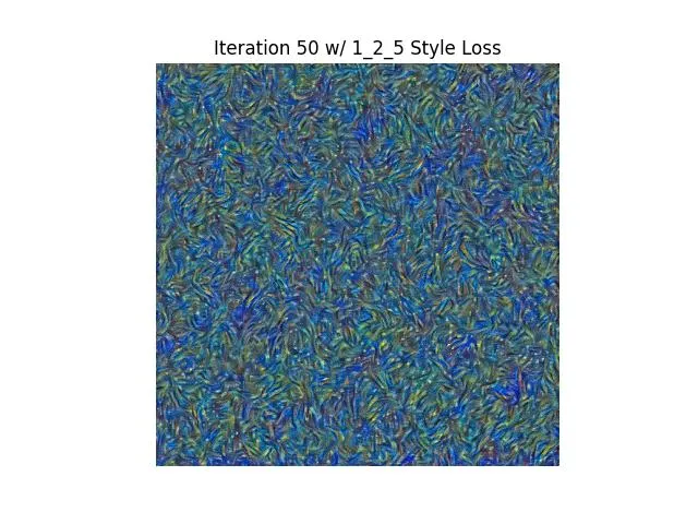 | 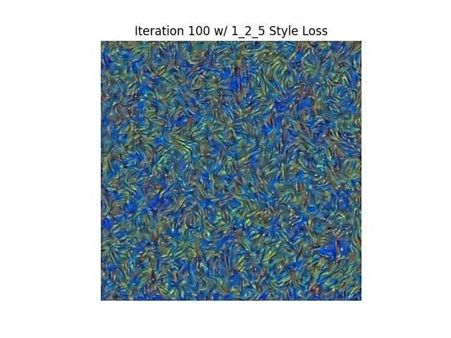 | 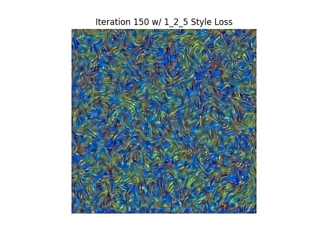 | 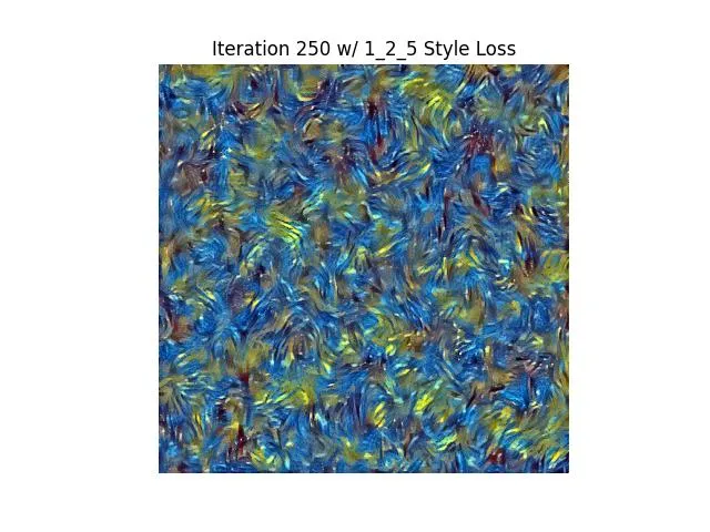 | 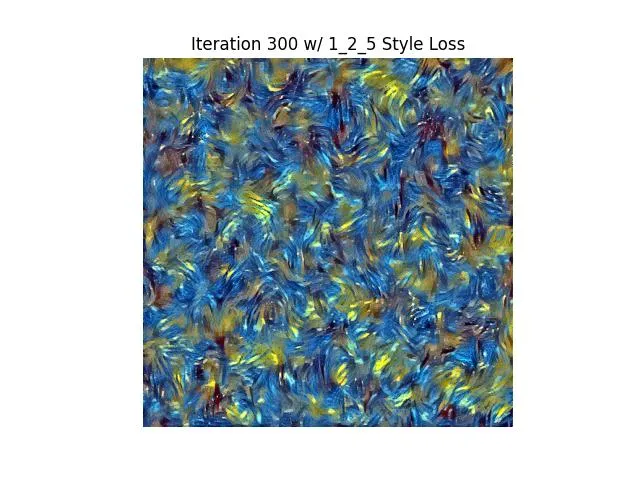 |
| 13 | 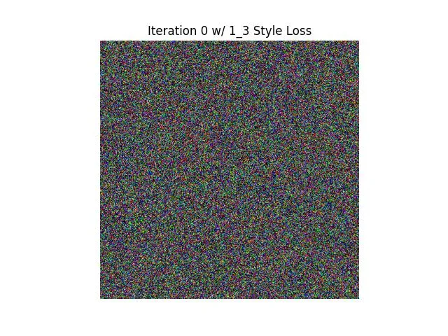 | 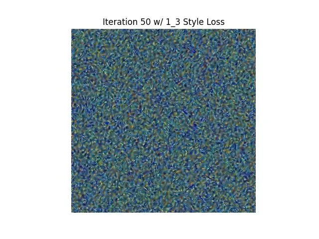 | 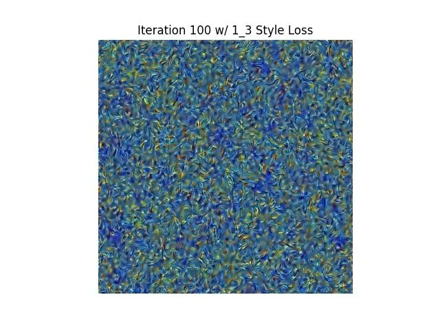 | 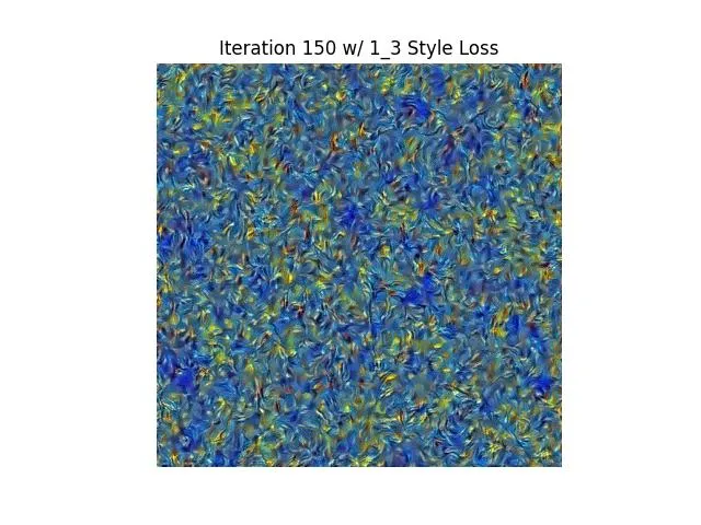 | 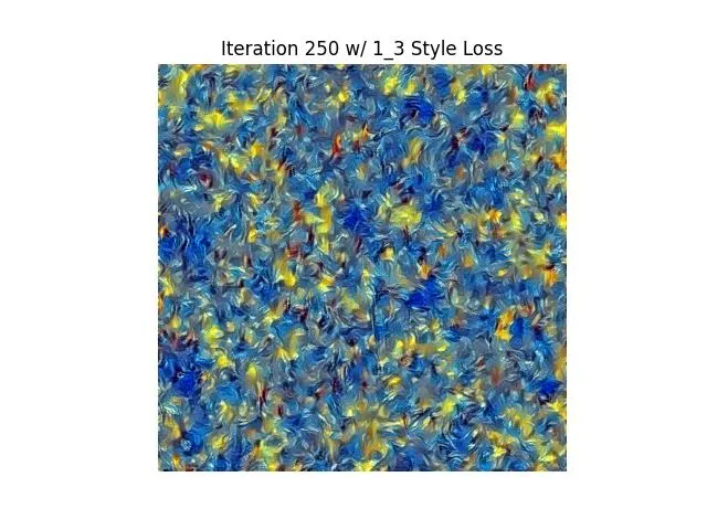 | 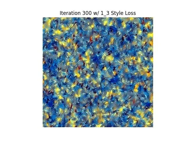 |
| 134 | 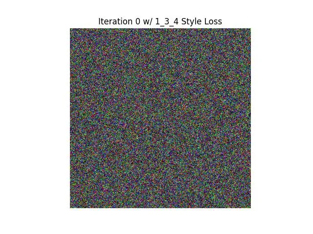 | 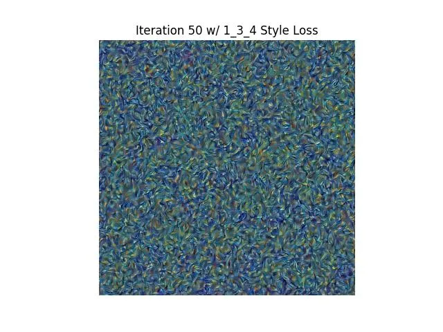 | 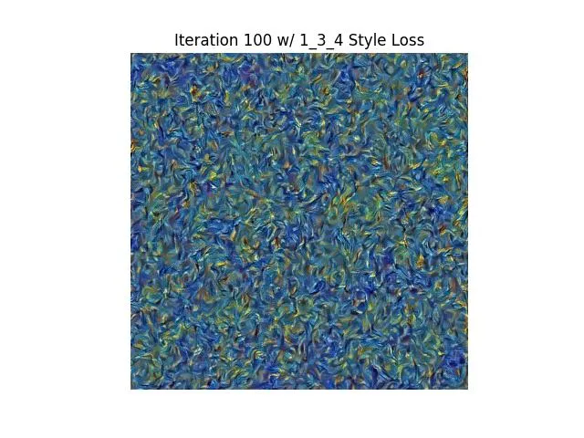 | 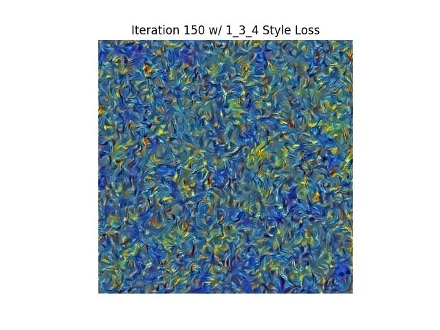 | 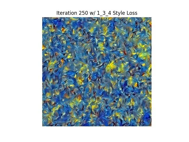 | 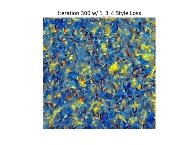 |
| 1345 |  | 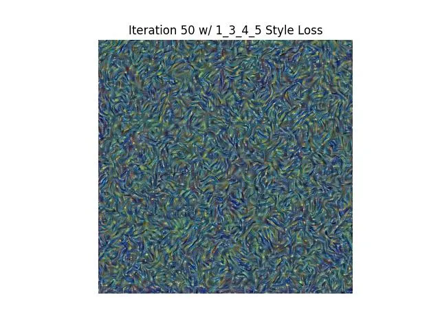 | 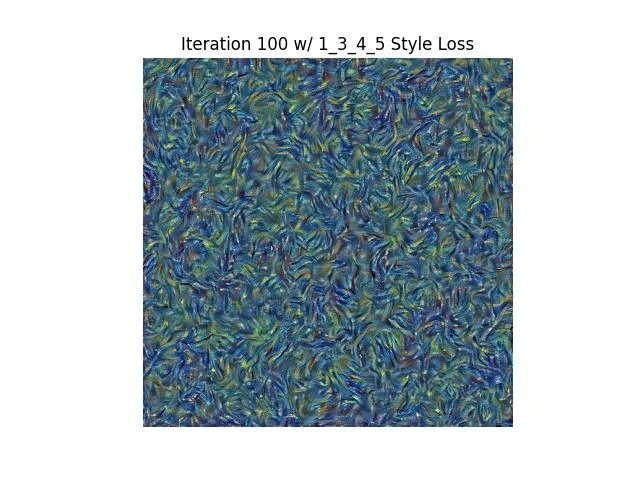 | 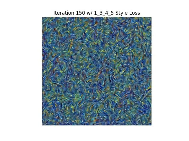 | 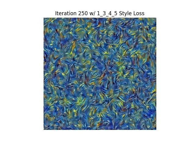 | 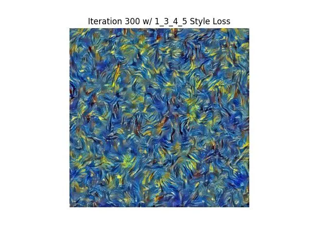 |
| 135 | 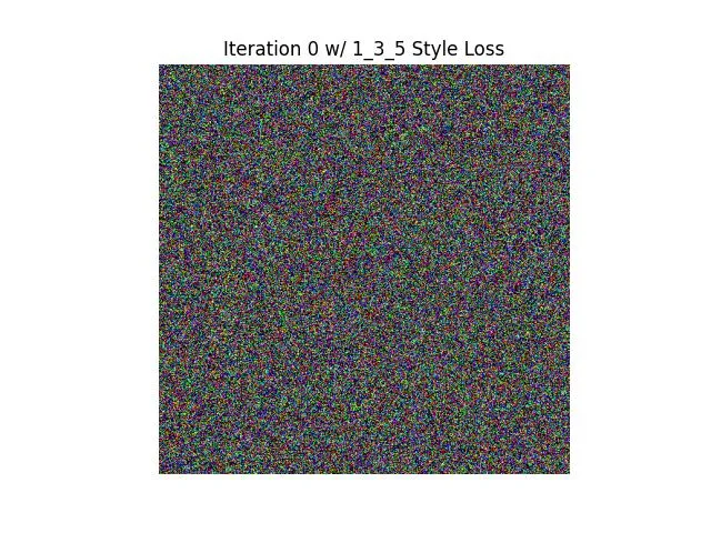 | 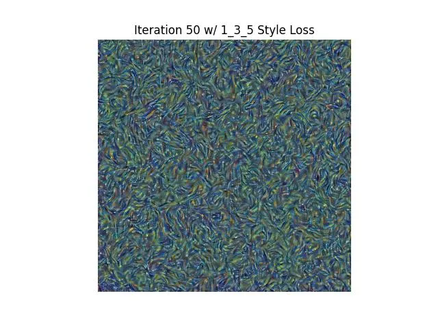 | 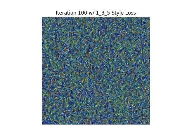 | 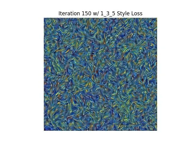 | 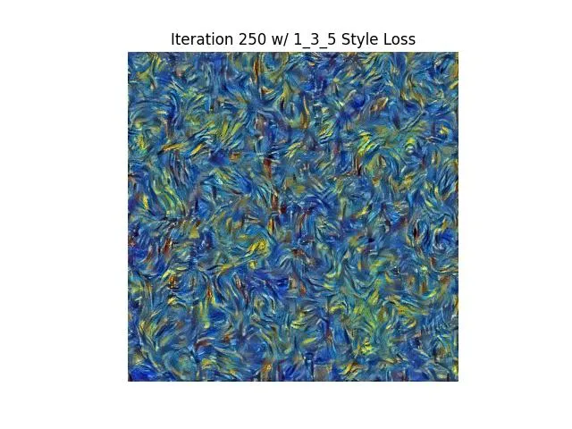 | 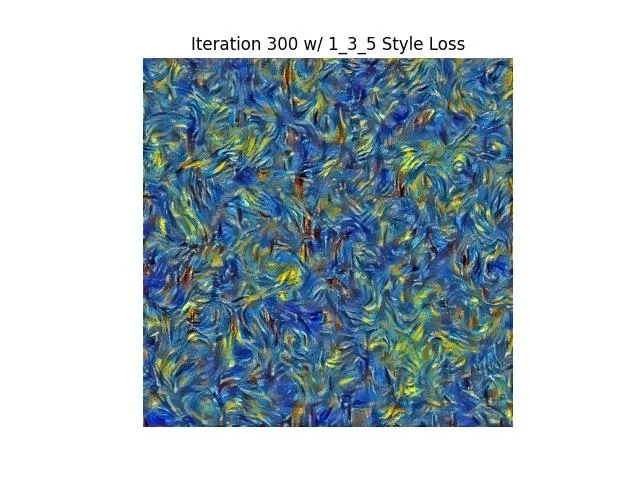 |
| 14 | 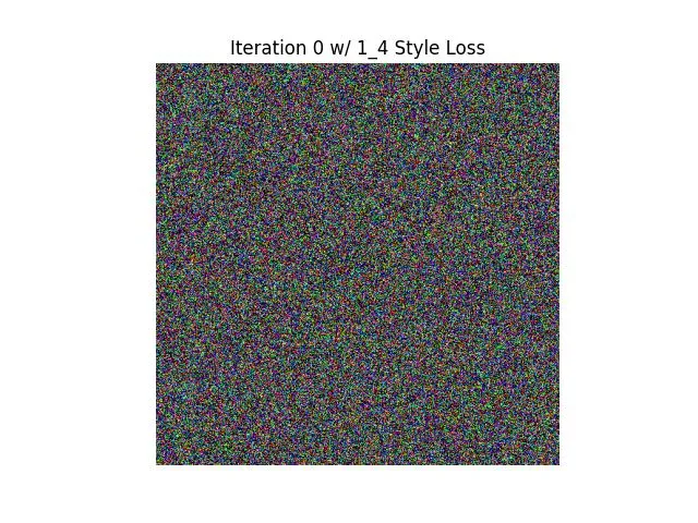 | 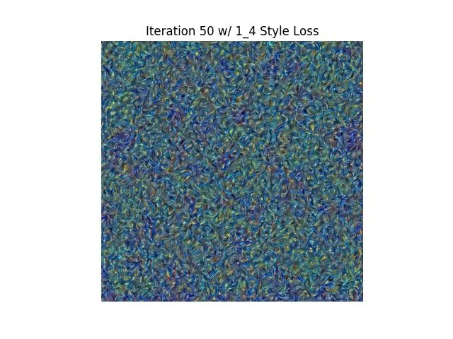 | 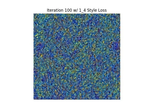 | 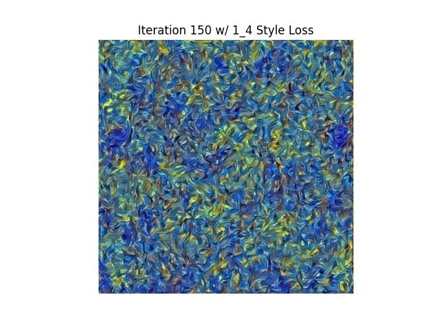 | 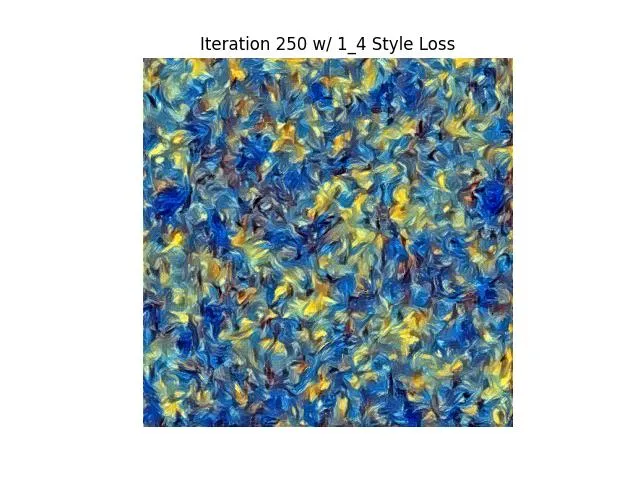 | 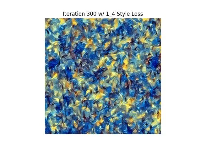 |
| 145 | 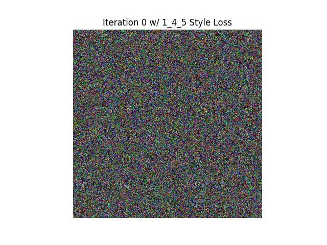 | 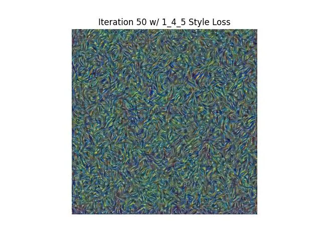 | 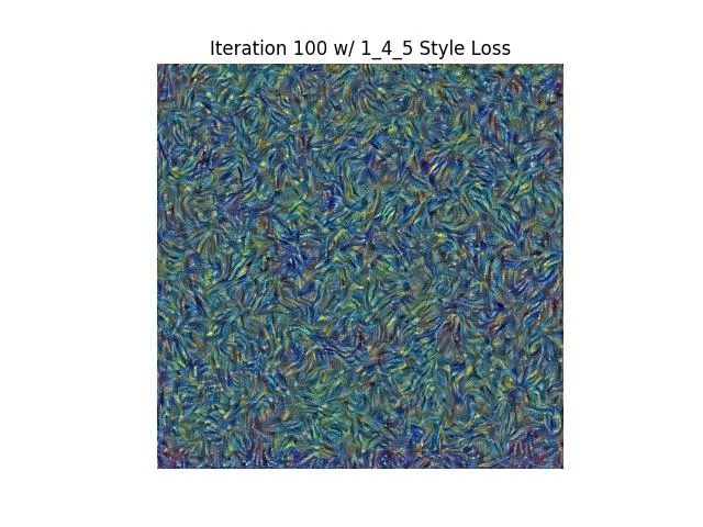 | 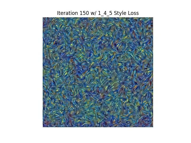 | 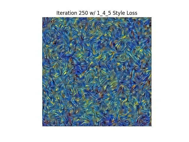 | 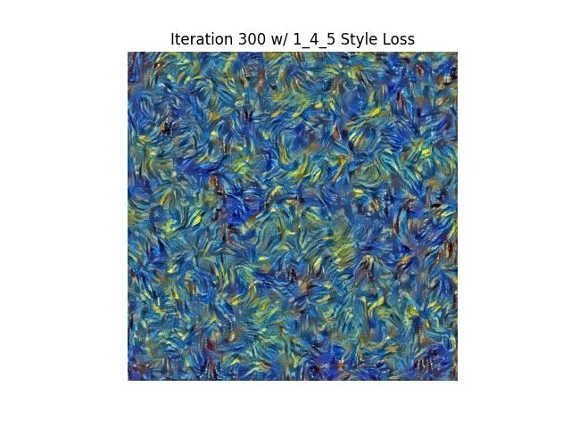 |
| 15 | 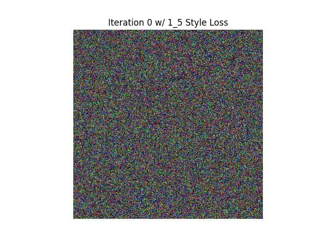 | 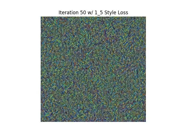 | 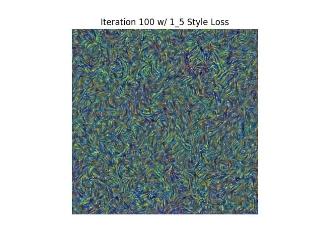 | 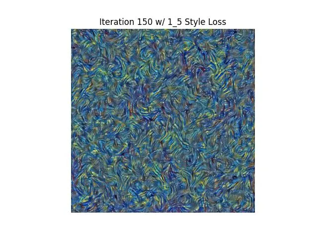 | 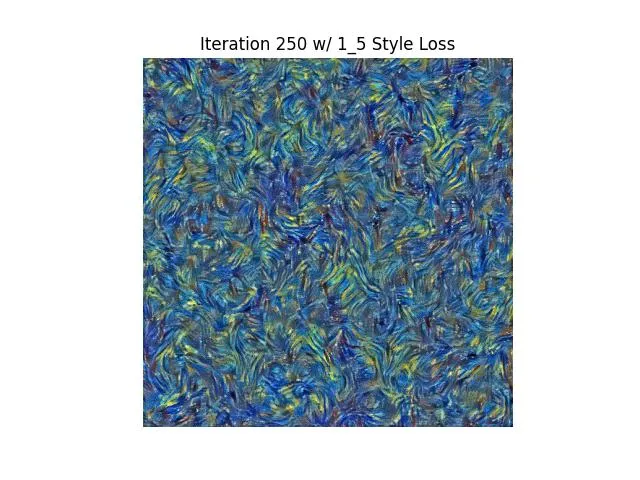 | 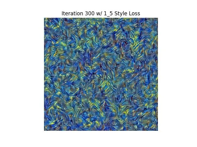 |
| 2 | 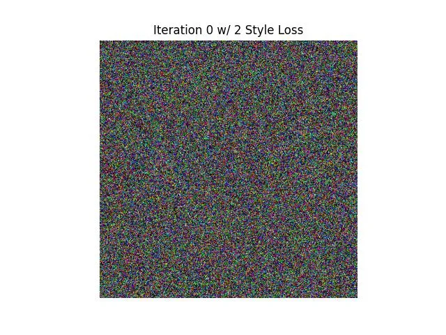 | 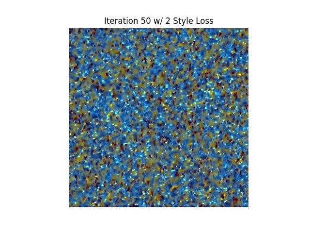 | 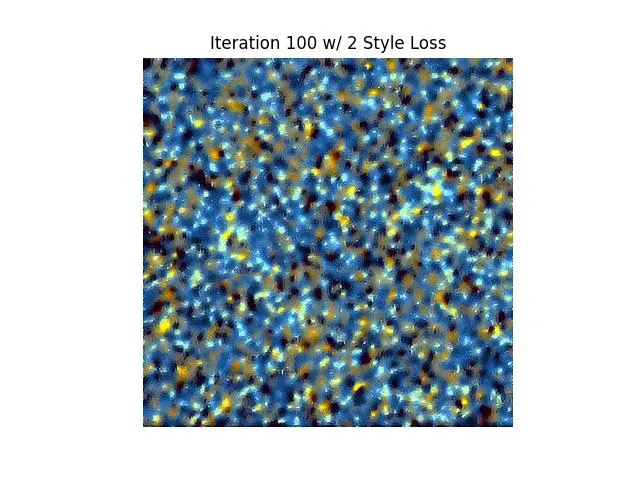 | 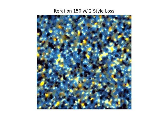 | 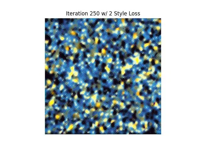 | 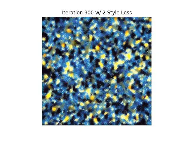 |
| 23 | 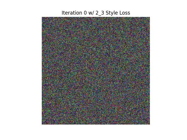 | 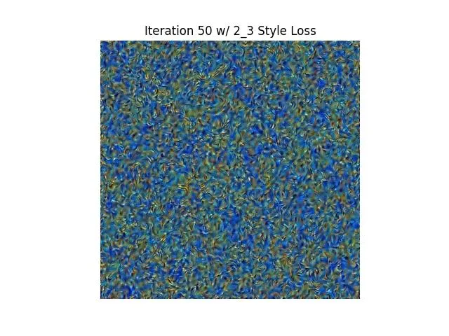 | 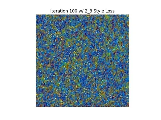 | 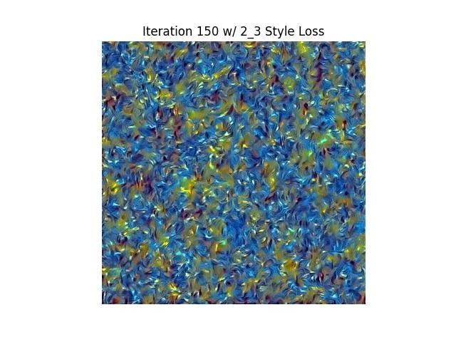 | 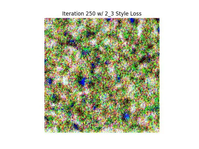 | 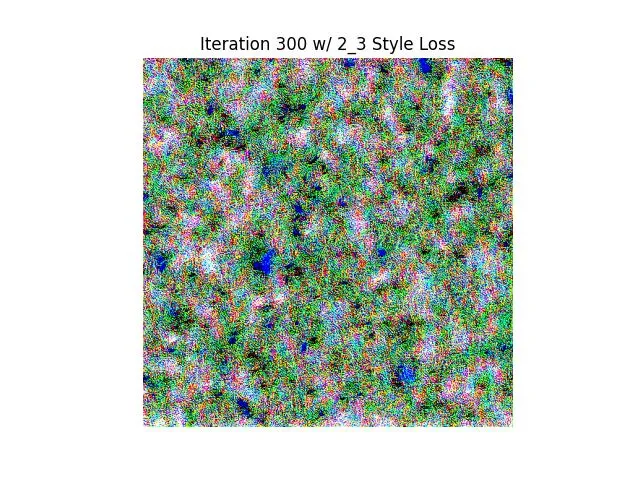 |
| 234 | 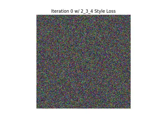 | 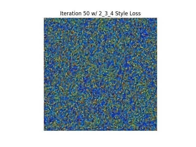 | 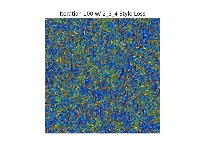 | 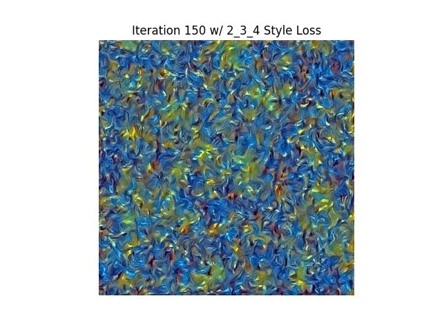 | 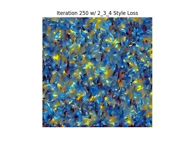 | 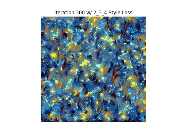 |
| 2345 | 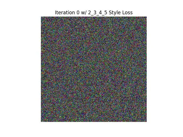 | 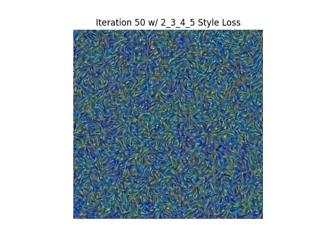 | 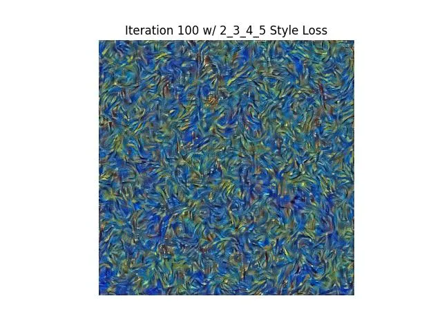 | 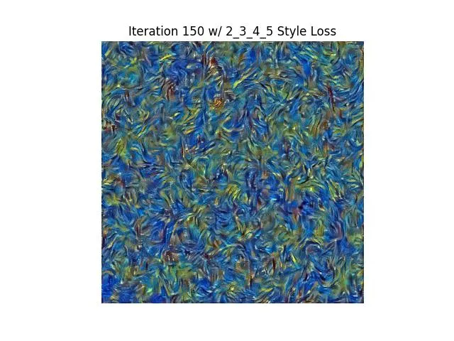 | 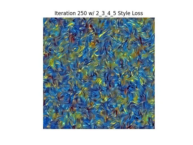 | 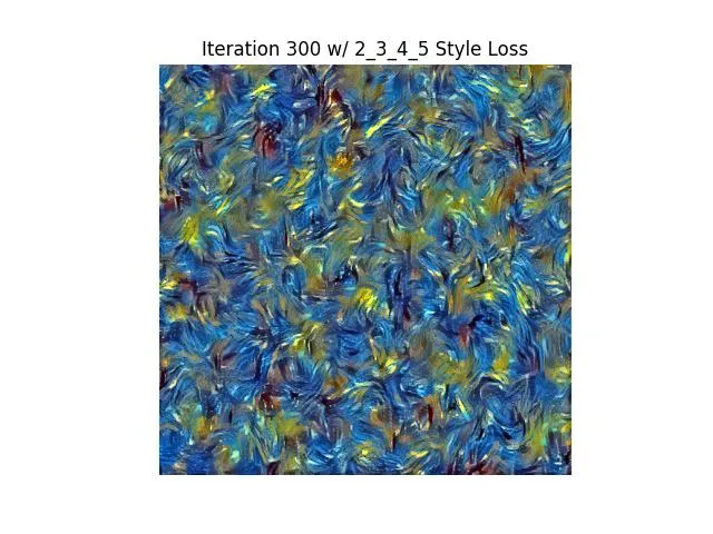 |
| 235 | 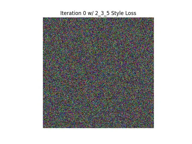 | 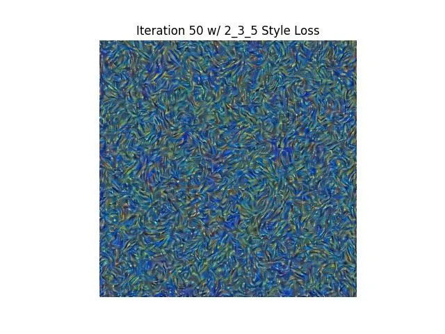 | 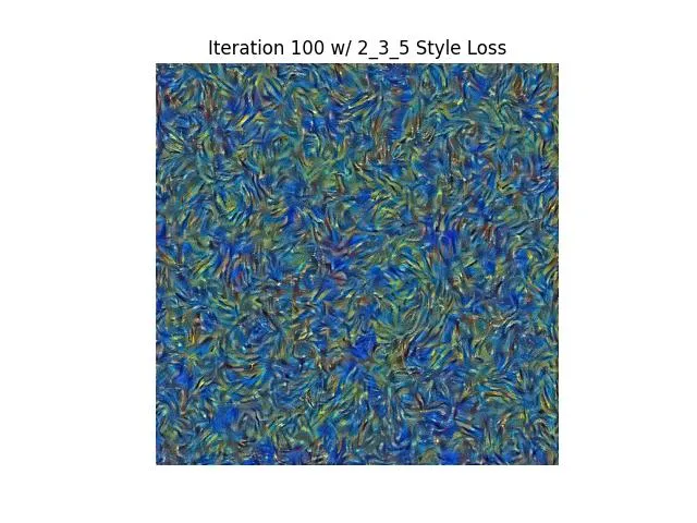 | 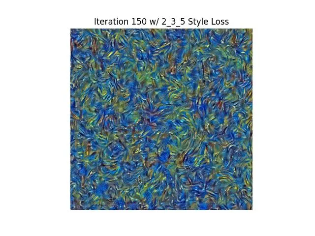 | 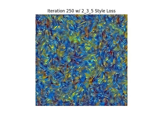 | 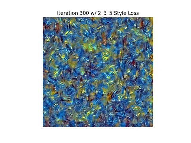 |
| 24 | 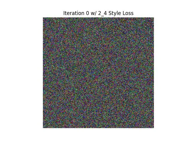 | 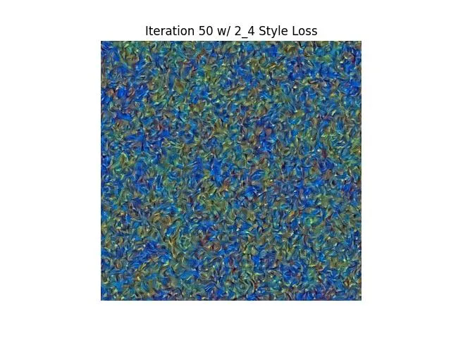 | 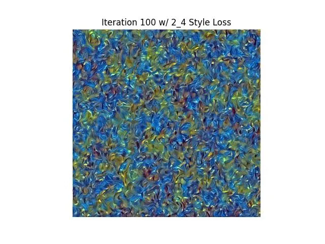 | 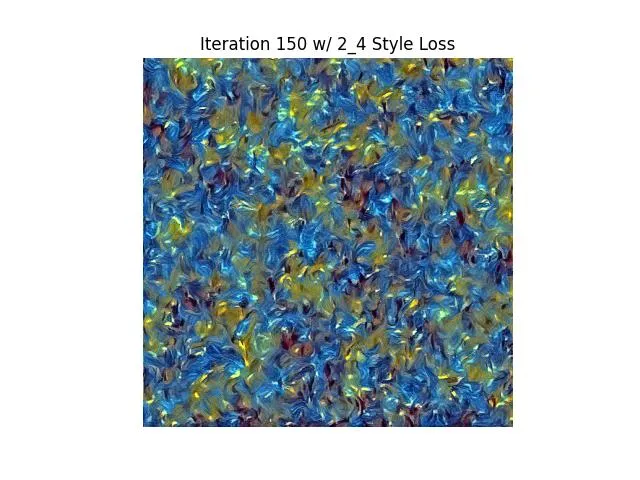 | 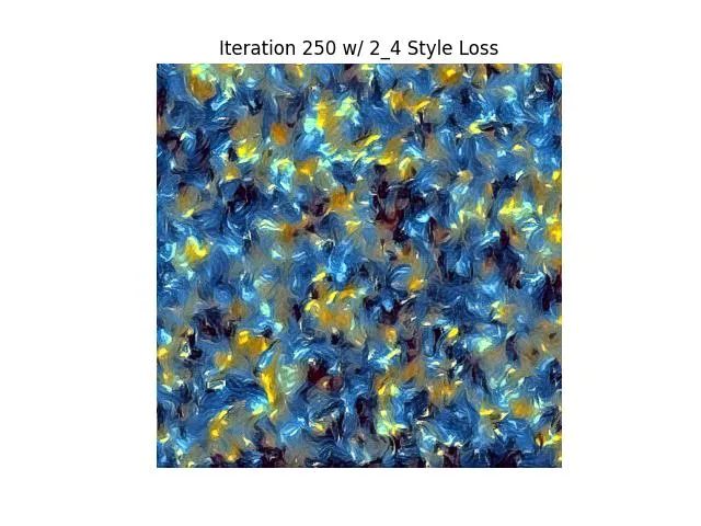 | 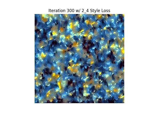 |
| 245 | 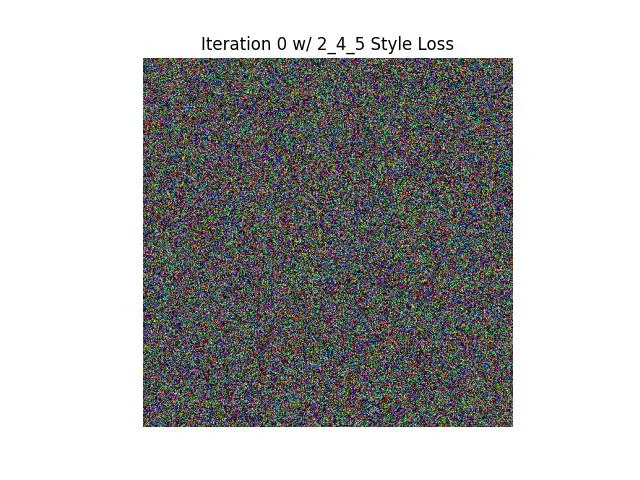 | 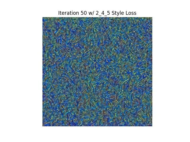 | 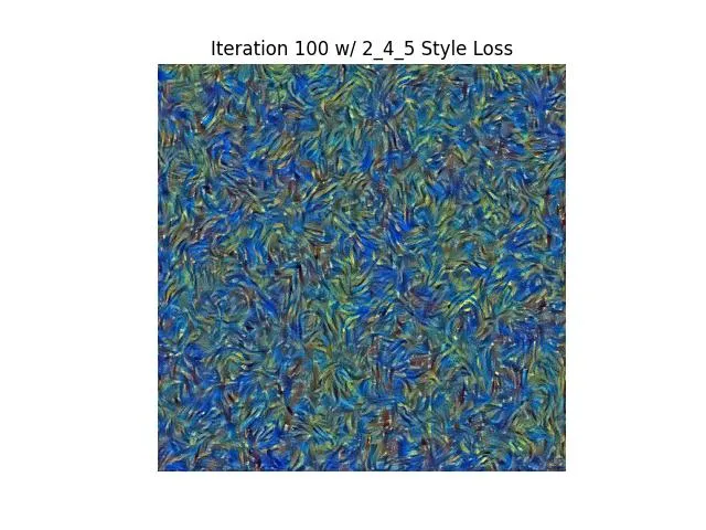 | 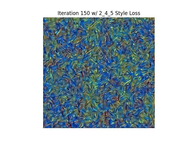 | 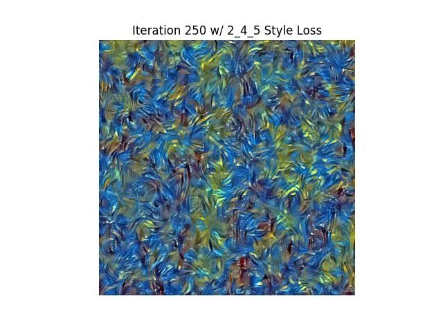 | 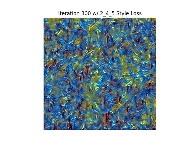 |
| 25 | 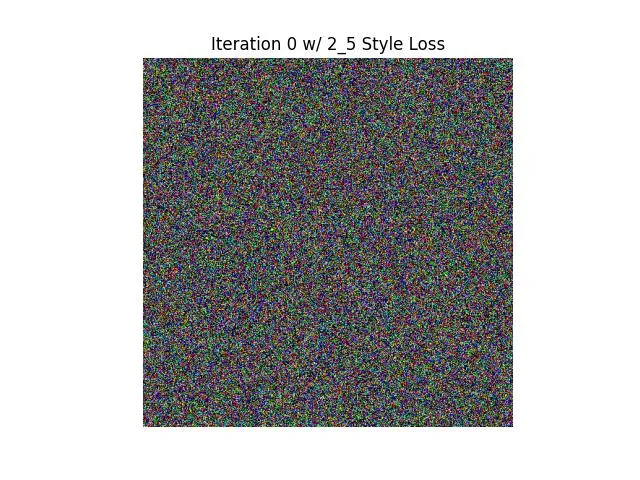 | 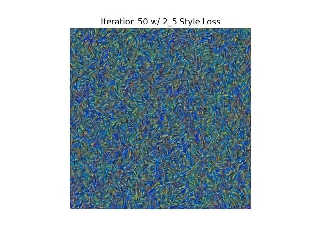 | 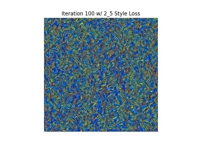 | 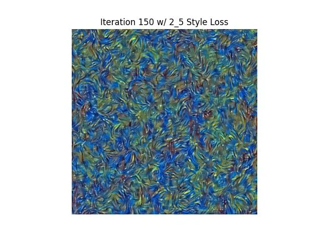 | 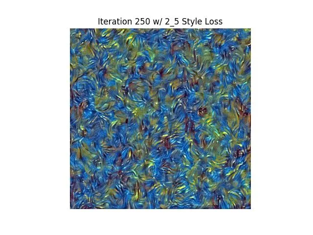 | 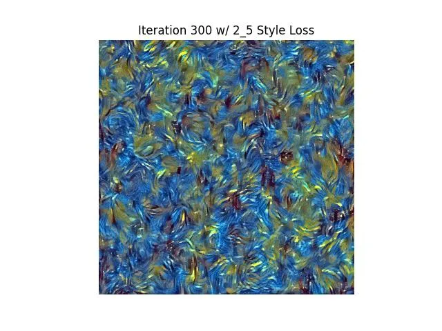 |
| 3 | 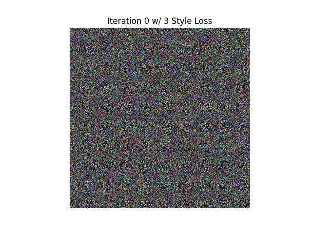 | 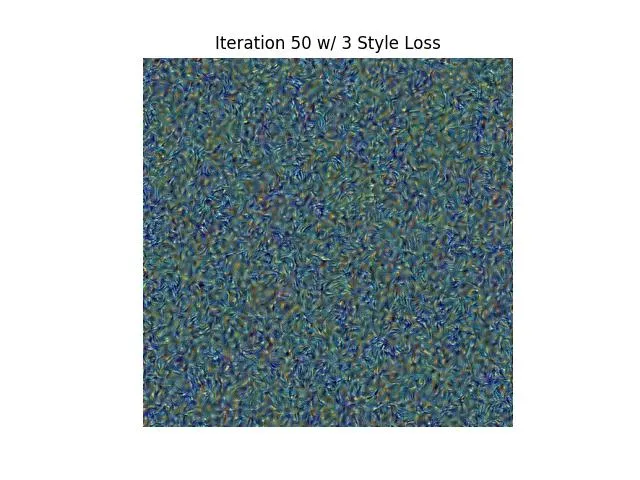 | 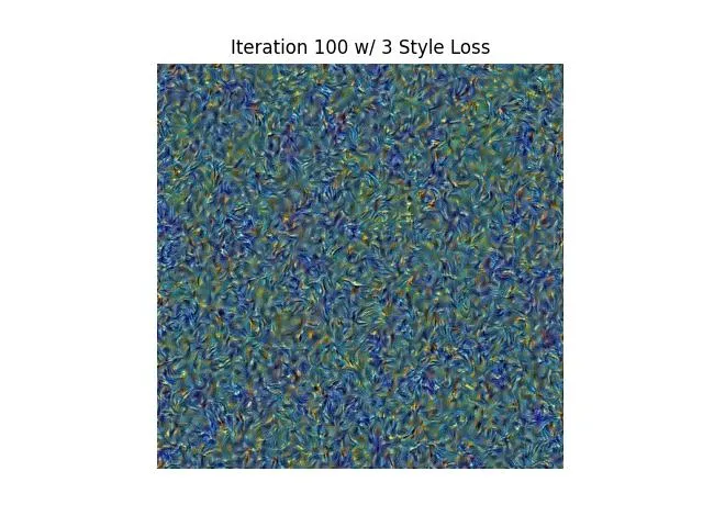 | 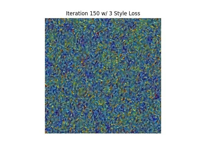 | 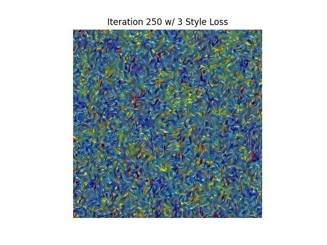 | 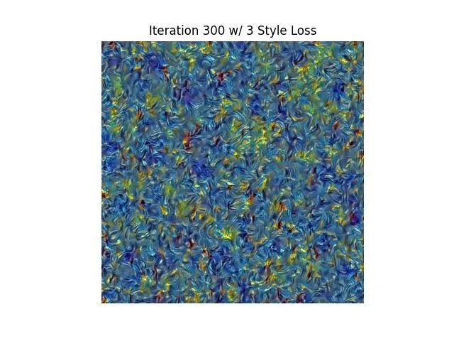 |
| 34 | 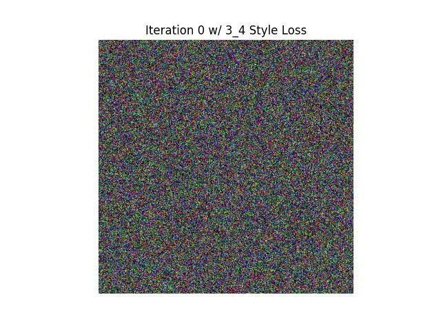 | 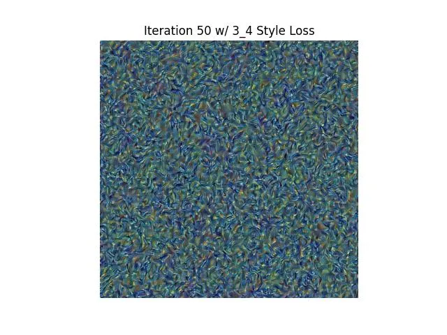 | 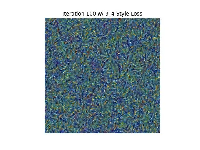 | 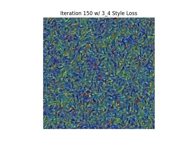 | 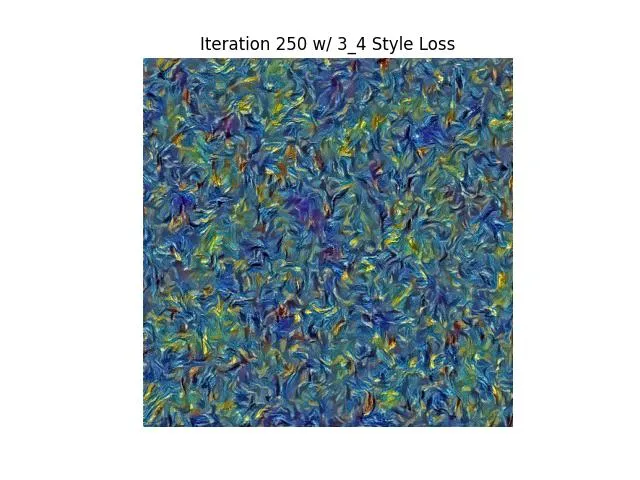 | 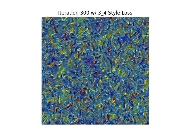 |
| 345 | 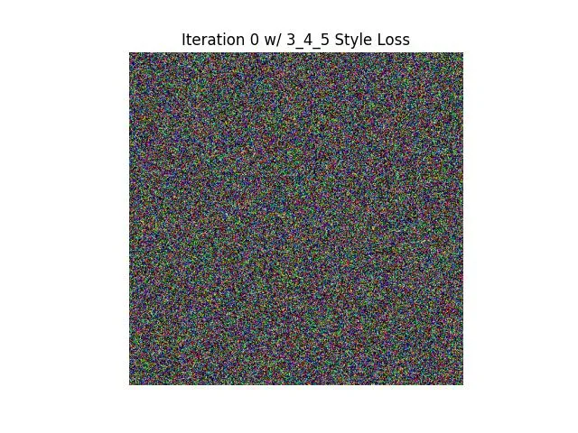 | 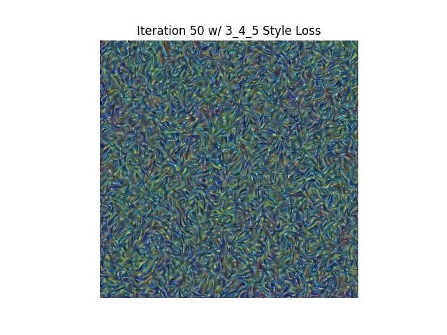 | 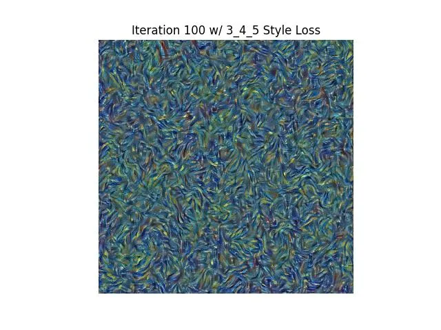 | 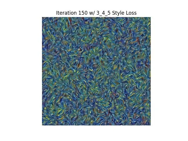 | 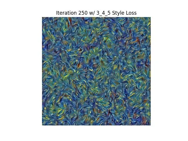 | 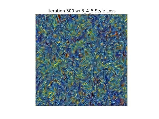 |
| 35 | 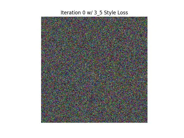 | 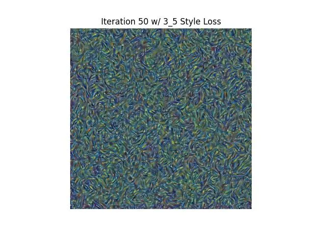 | 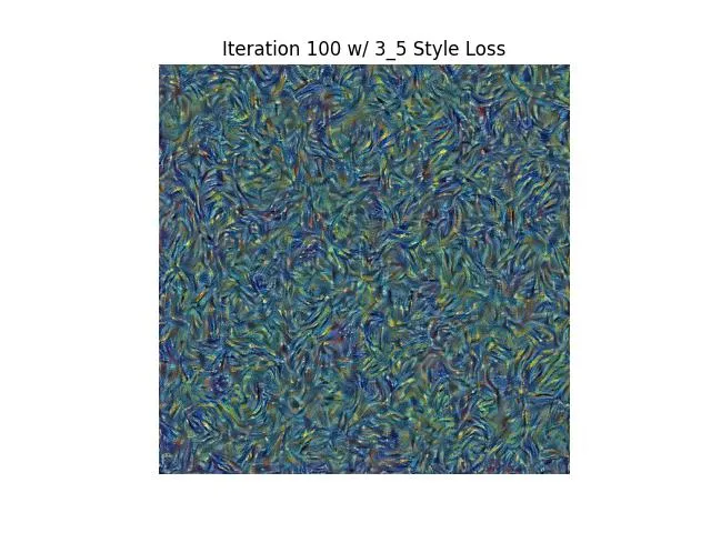 | 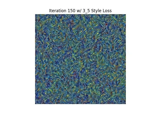 | 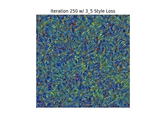 | 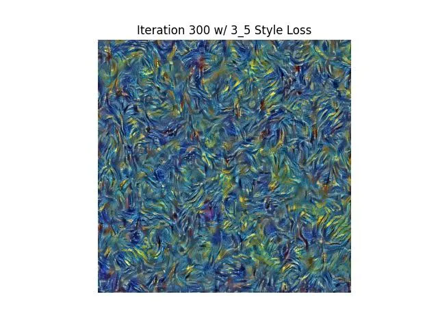 |
| 4 | 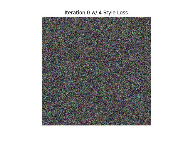 | 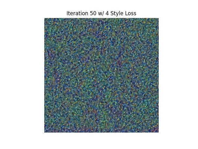 | 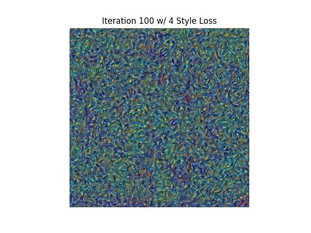 | 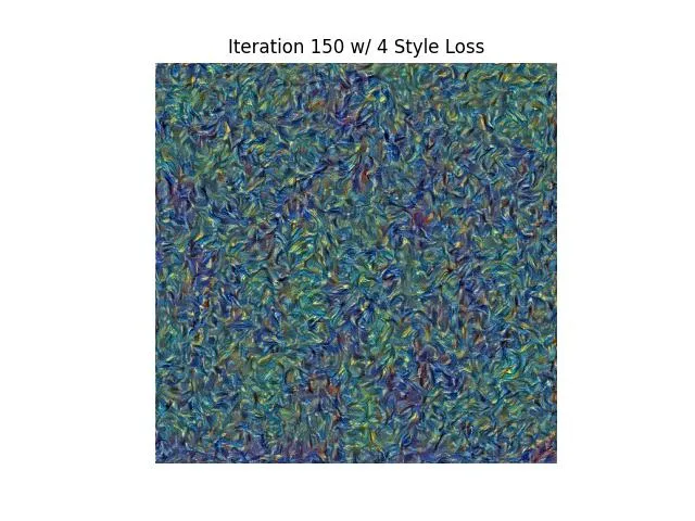 | 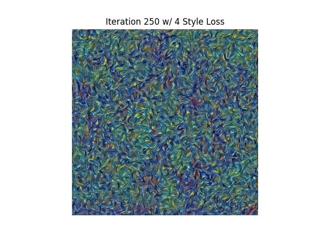 | 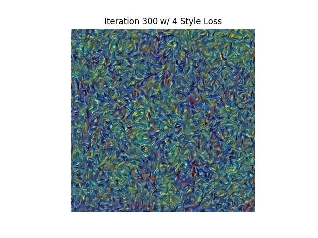 |
| 45 |  | 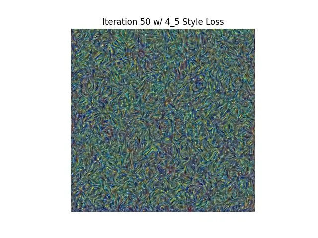 | 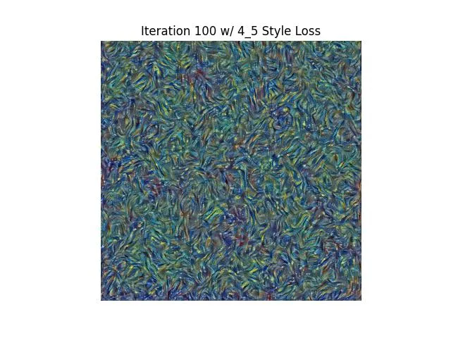 | 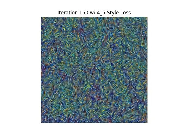 | 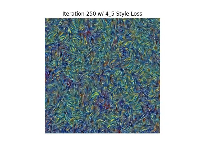 | 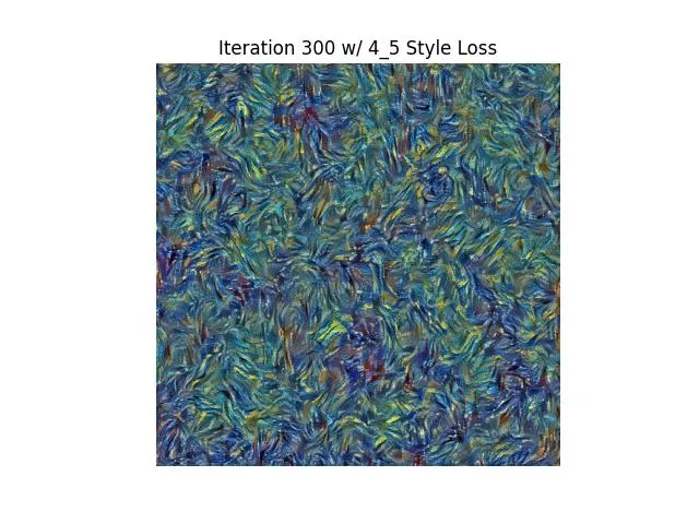 |
| 5 | 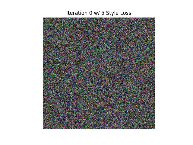 | 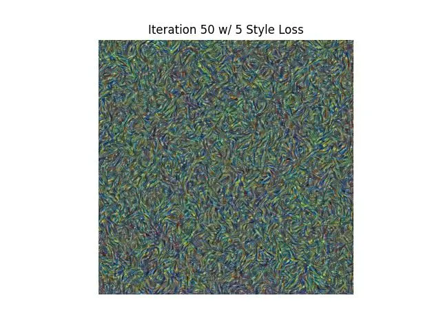 | 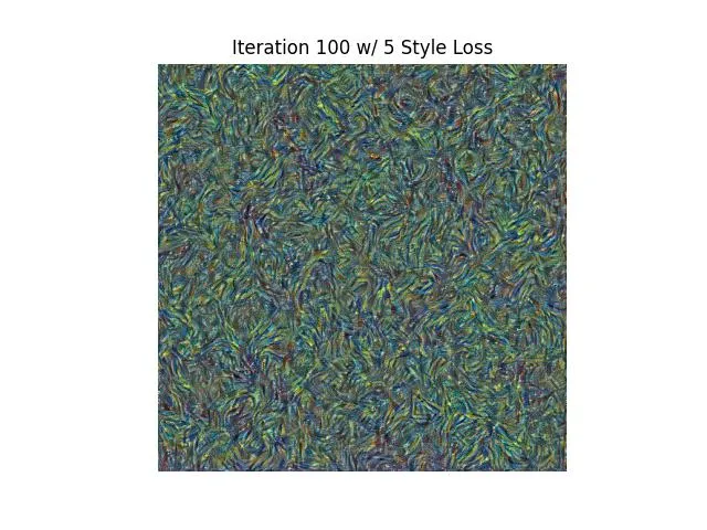 | 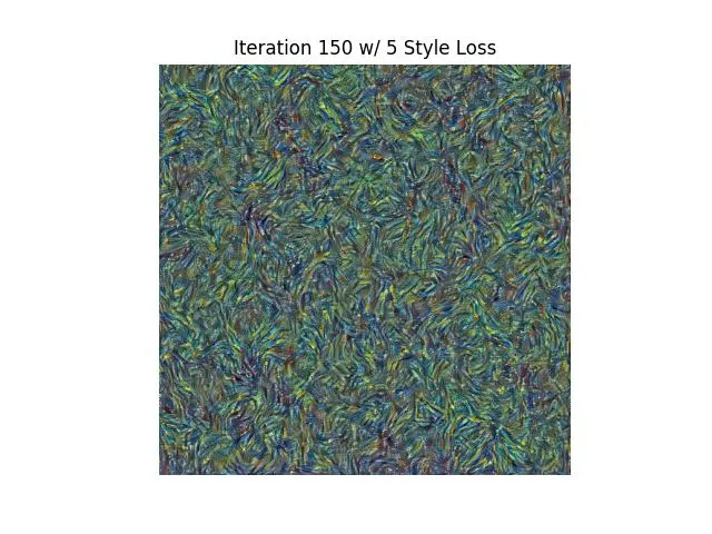 | 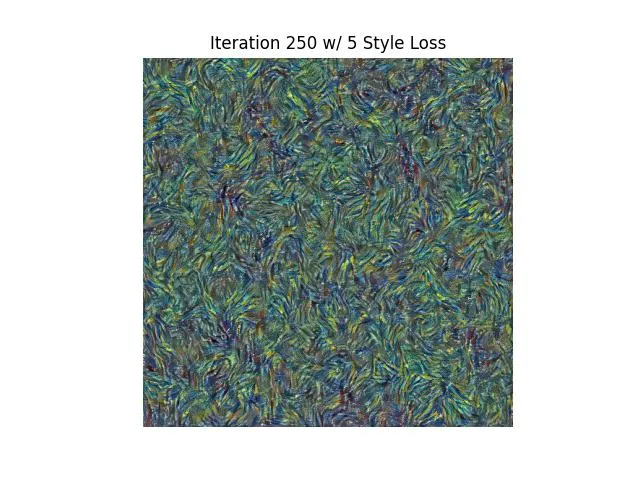 | 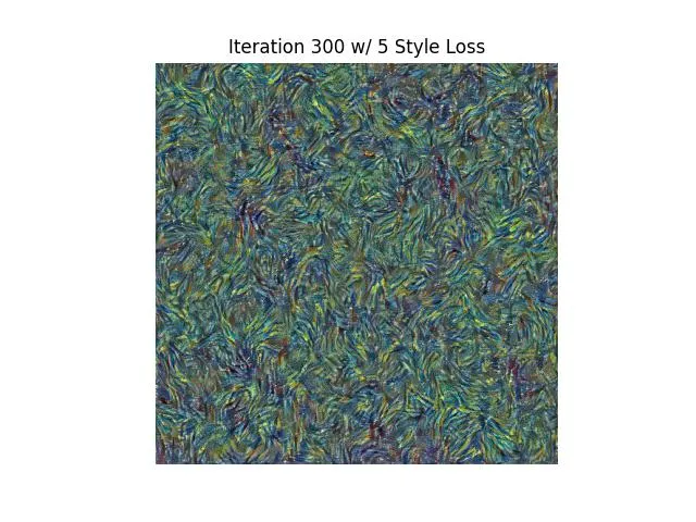 |
I ended up going with 1_3_4 just because I liked it. For reference, 1_3_4 had a style loss of 3.466813 after 300 iterations while 1_2_3_4_5 the initial default
iteration had a loss of 14.167436 after 300 iterations. There were experiments with lower losses like 1_2_3_4 with 2.999 or 1_2_4 with 1.36 but I didn’t like the look
as much.
I think that each layer captures more of the higher or lowever levels of style details which makes sense. As you go from top to bottom the details go from coarser to finer showing the effects of deeper layers.
Texture Synthesis Results
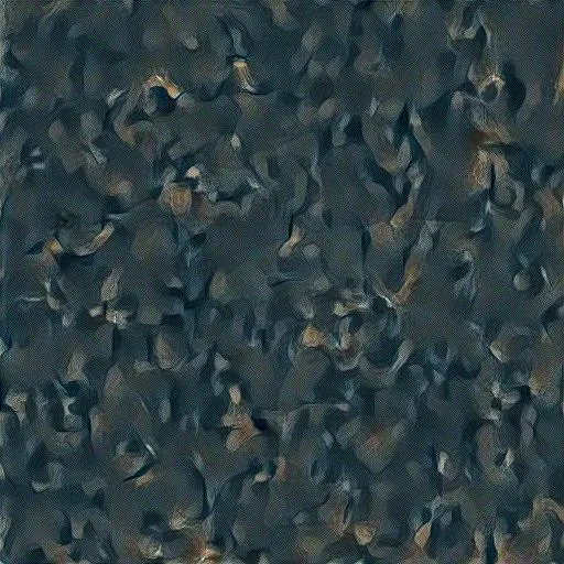
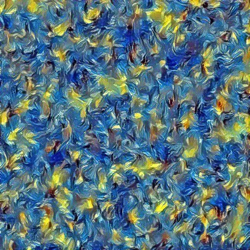
Similar to the content loss experiments above here is texture synthesis run on two noise patterns.
| Noise Type | 0 | 50 | 100 | 150 | 200 | 250 | 300 |
|---|---|---|---|---|---|---|---|
| Noise 2 | 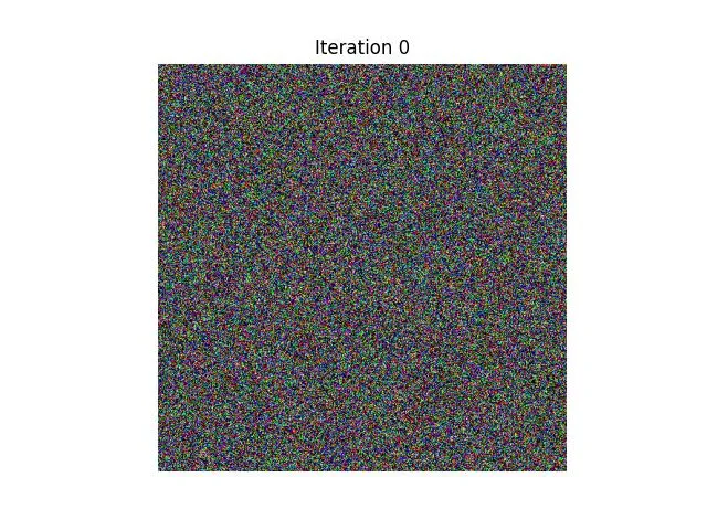 | 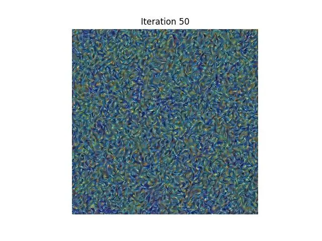 | 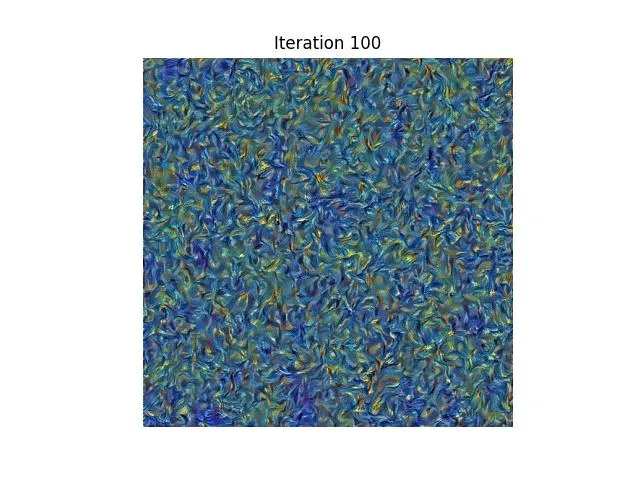 | 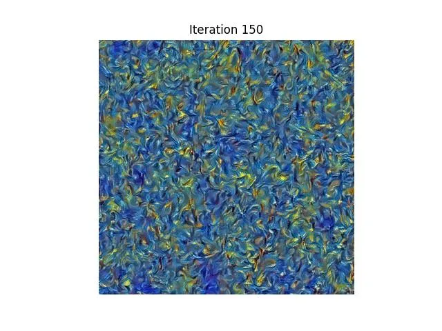 | 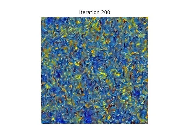 | 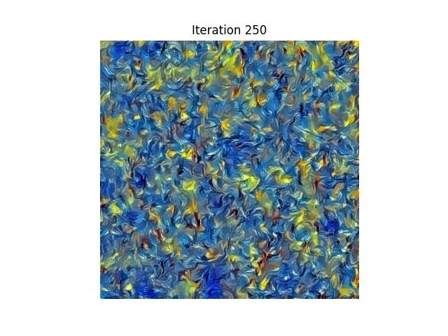 | 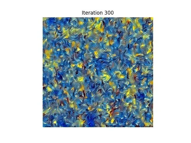 |
| Noise 3 | 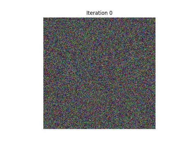 | 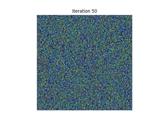 | 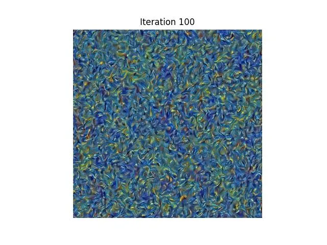 | 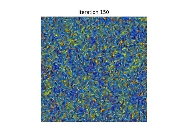 | 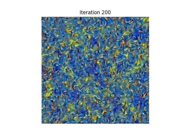 | 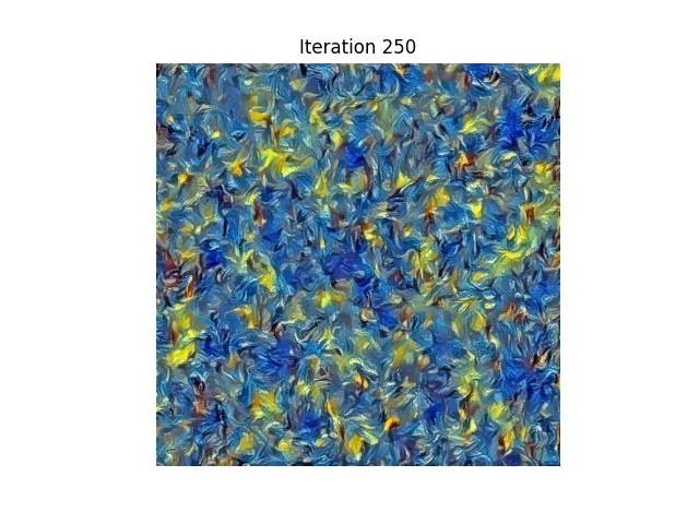 | 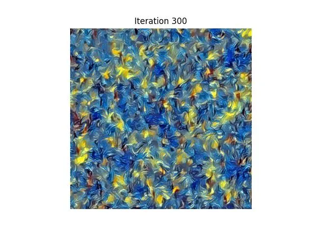 |
| Name | 50 | 100 | 150 | 200 | 250 | 300 |
|---|---|---|---|---|---|---|
| Noise 1 | 37.577023 | 16.584526 | 10.589894 | 7.149663 | 5.04898 | 3.749736 |
| Noise 2 | 38.905602 | 16.395645 | 10.272487 | 7.053143 | 4.767246 | 3.256261 |
The L2 loss between the outputs was 307 which makes sense as there’s no reason for them to have a low pixel loss.
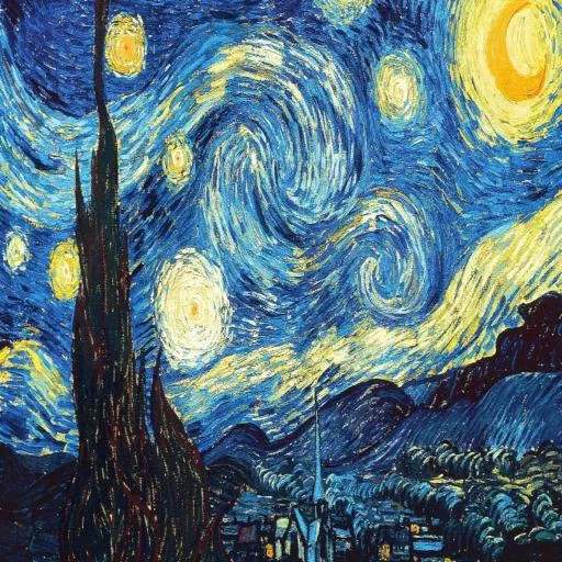
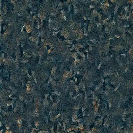
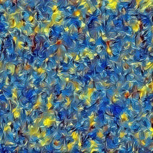
As you can see the texture differ in their layout but do indeed capture the starry night texture. Going forward I’ll use conv_1, conv_3, conv_4 to calculate style loss.
Hyperparameter Tuning
To figure out the hyper parameters for content and style weight I ran a
search over params
[1.e+00, 1.e+01, 1.e+02, 1.e+03, 1.e+04, 1.e+05, 1.e+06, 1.e+07, 1.e+08]
for style_weight and content_weight.
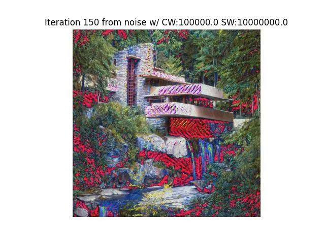
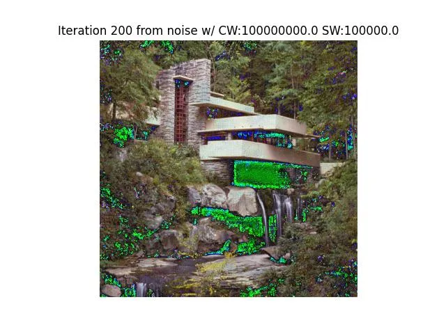
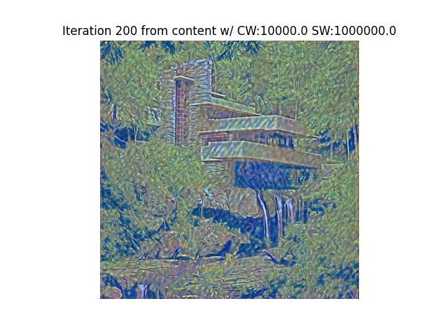
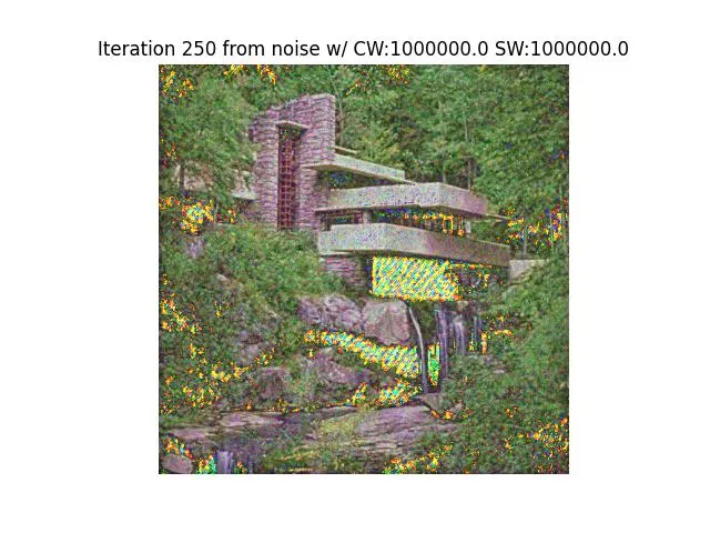
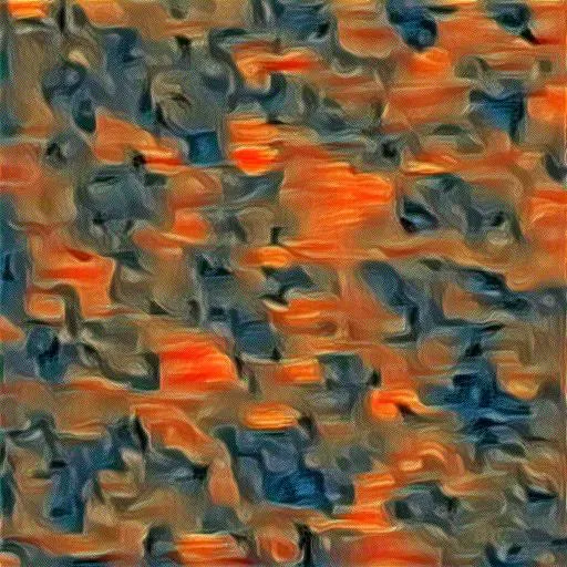
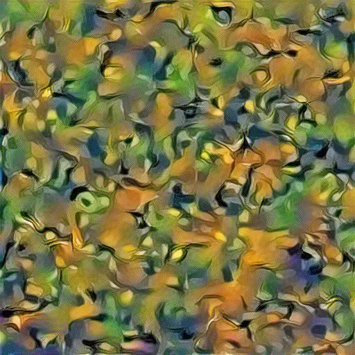
This generated a lot of images and a lot of optimizer instability at weird ratios. In retrospect it would’ve made more sense to have just do a search over the relative ratios of weight and style. That said, I would’ve never discovered the optimizer instability.
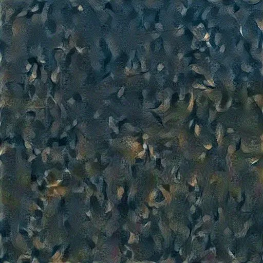
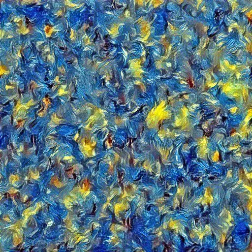
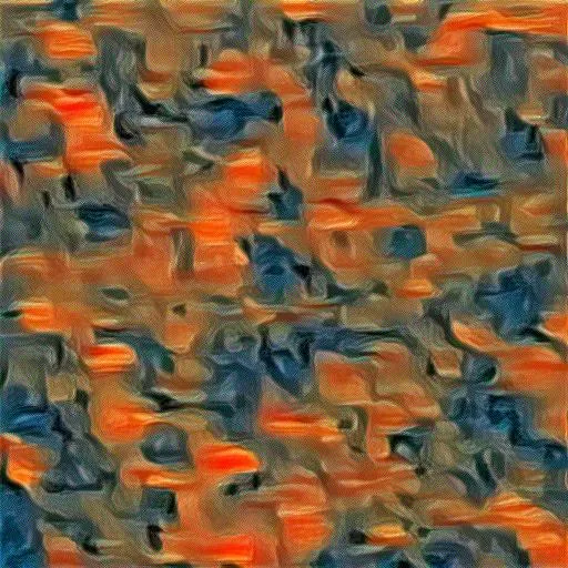
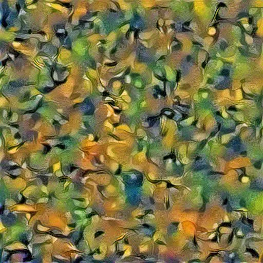
Below are some of the weird results.
I settled on relative ratios of content_weights = 1, style_weights = 1000000
Final Results
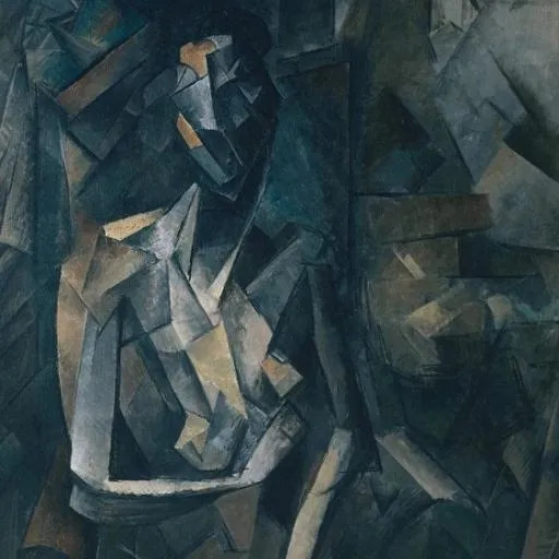
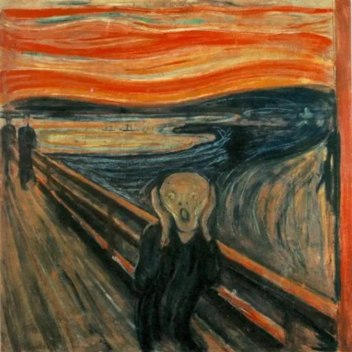
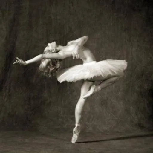
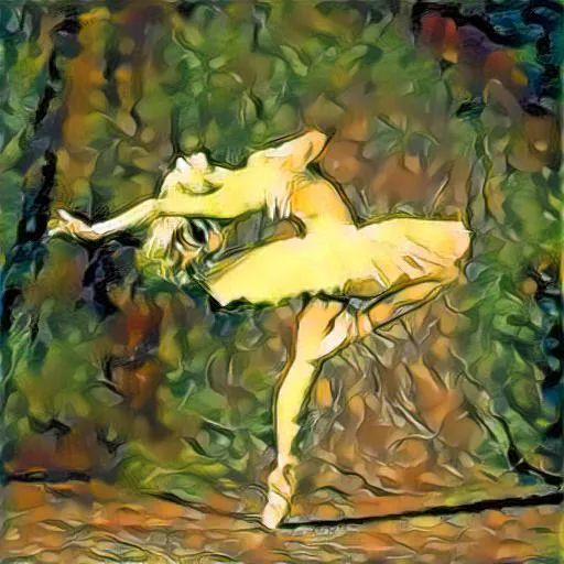
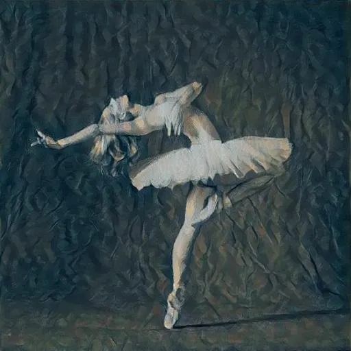
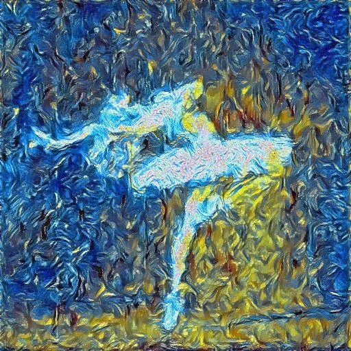
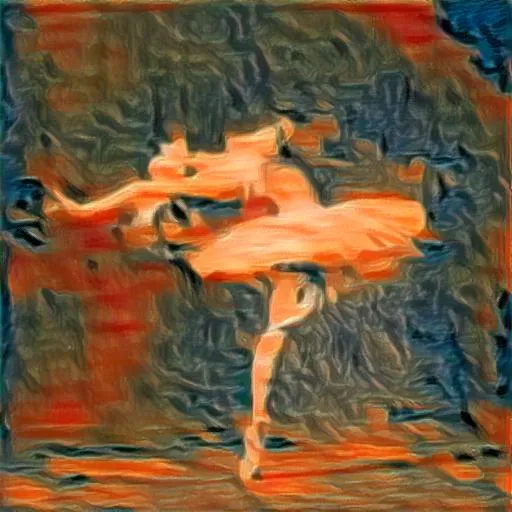
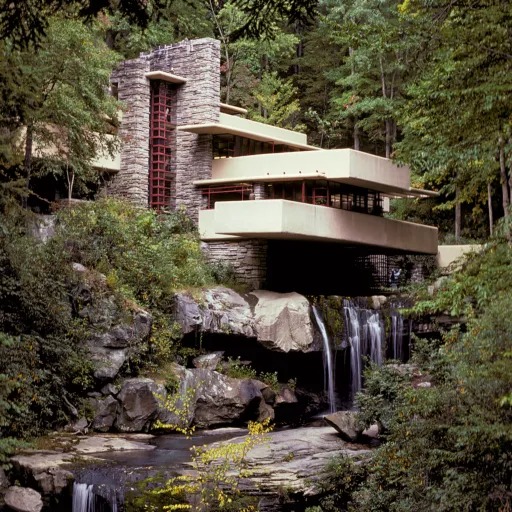
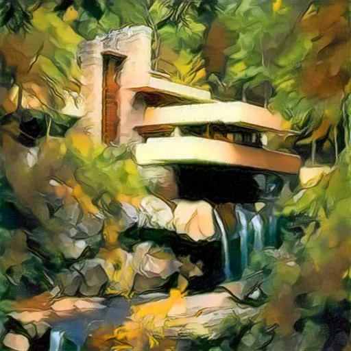
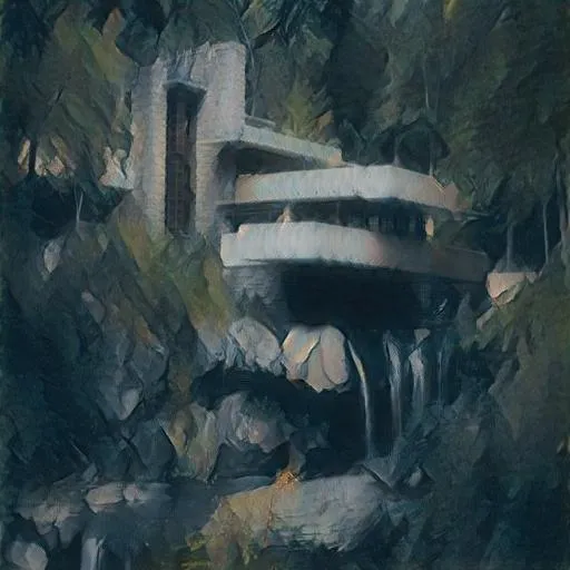
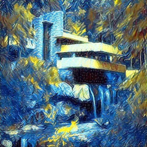
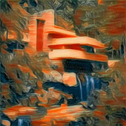
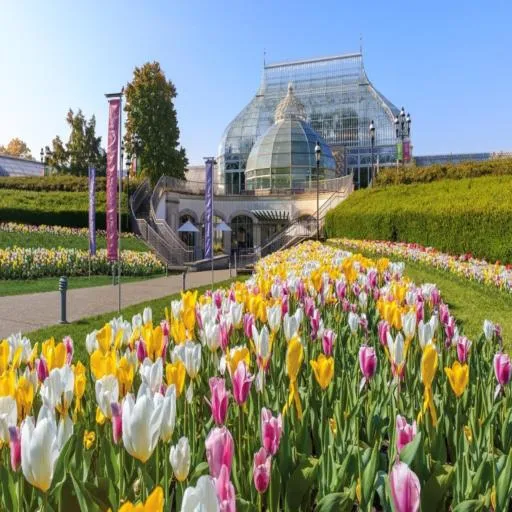
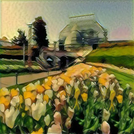
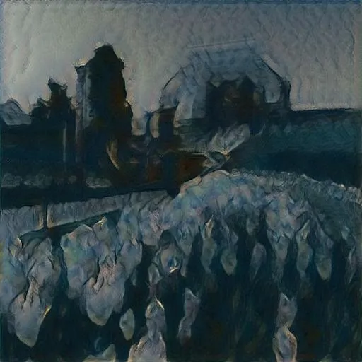
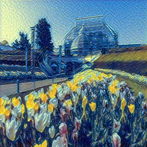
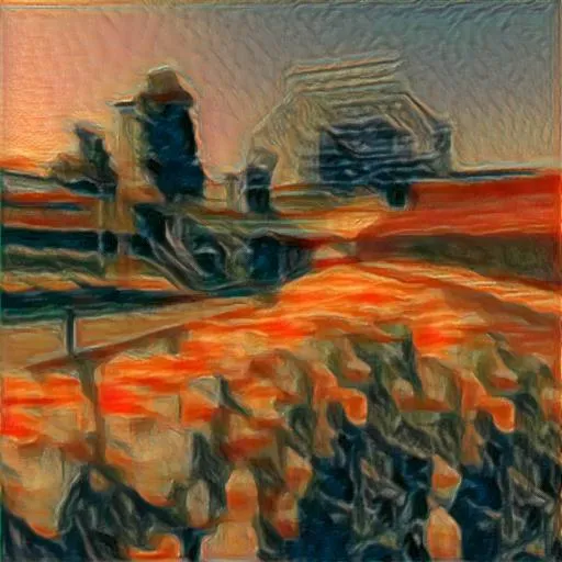
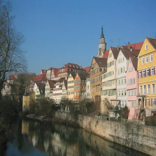
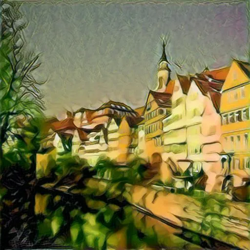
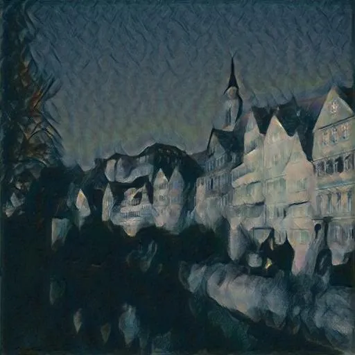
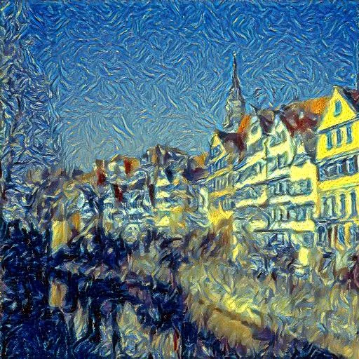
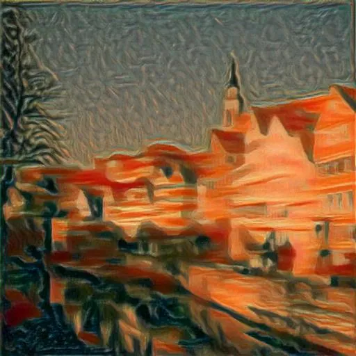
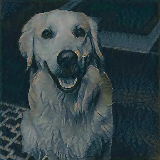
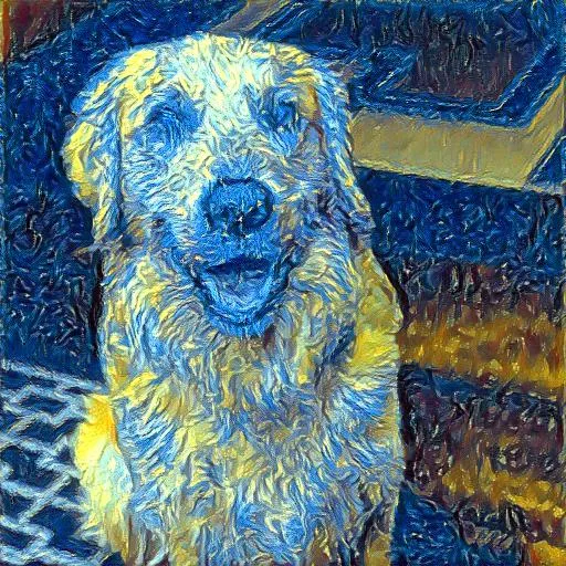
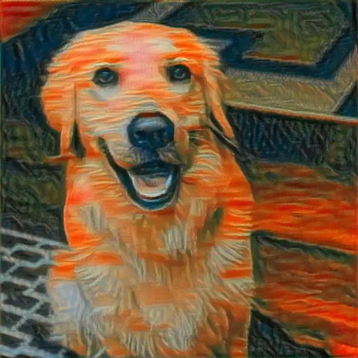
Below are the final results with all the previous experiments.
Content Initialization
 |  |  |  | |
|---|---|---|---|---|
 |  |  |  |  |
 |  |  |  |  |
 |  |  |  |  |
 |  |  |  |  |
 |  |  |  |  |
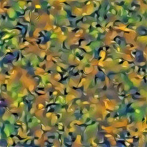
Noise Initialization
| | | | | |
|---|---|---|---|---|
| |  |  |  |  |
| |  |  |  |  |
| |  |  |  |  |
| |  |  |  |  |
| | 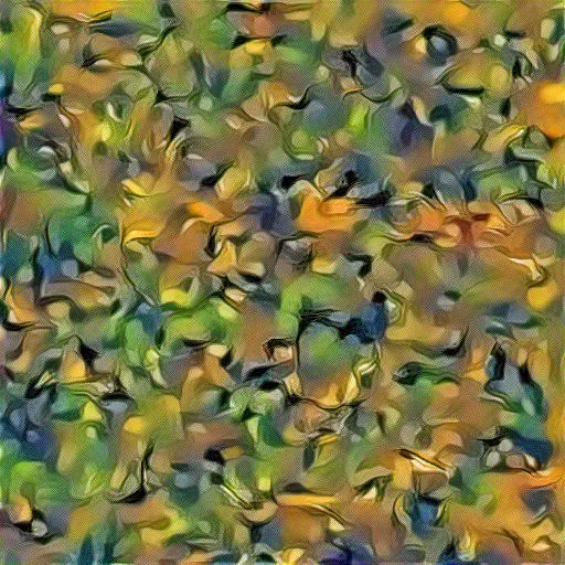 | 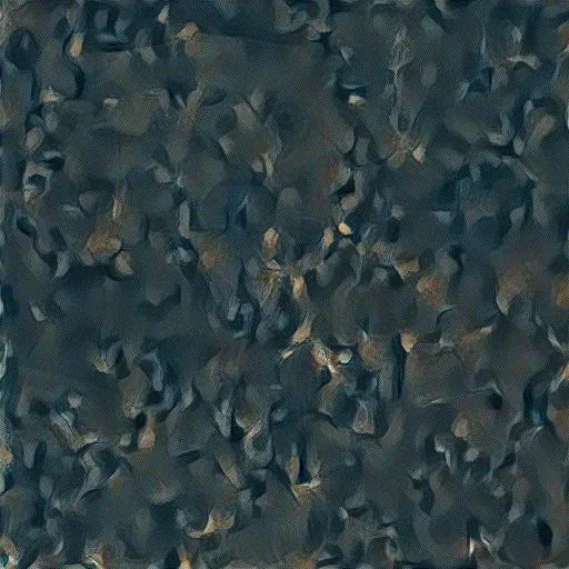 | 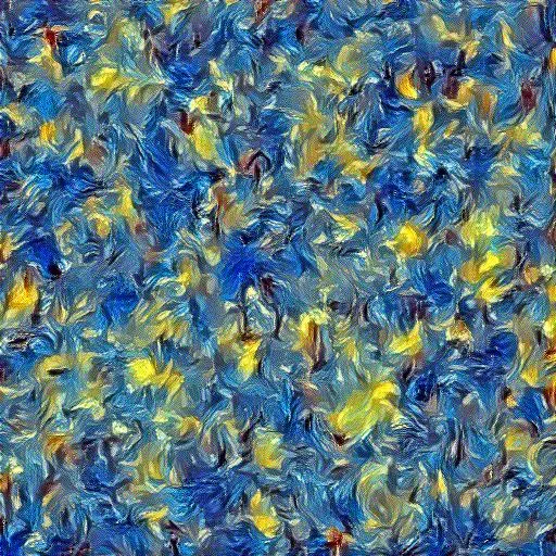 | 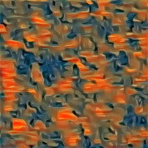 |
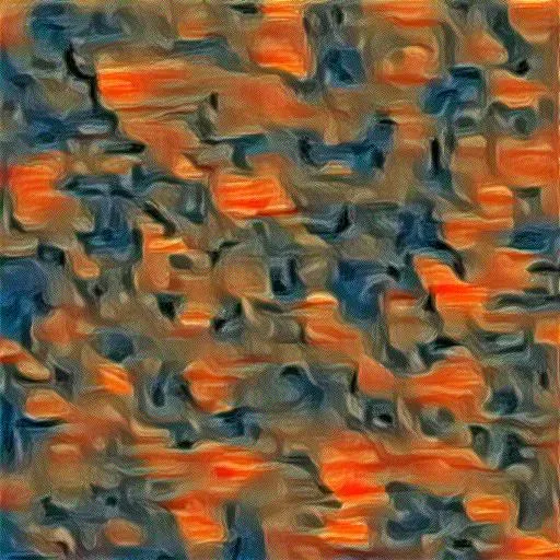
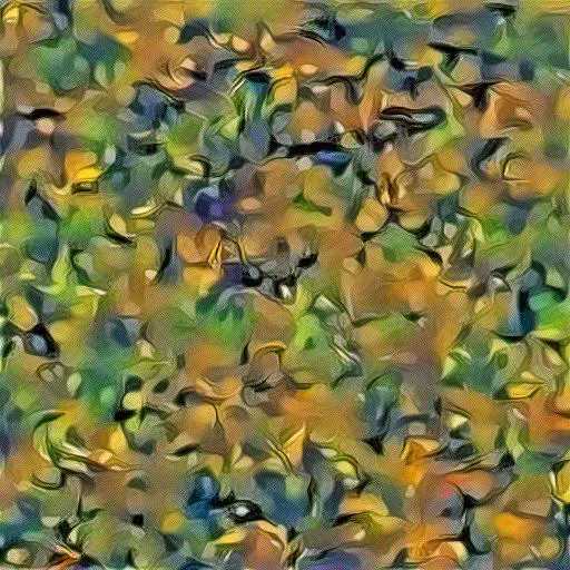
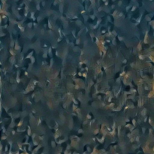
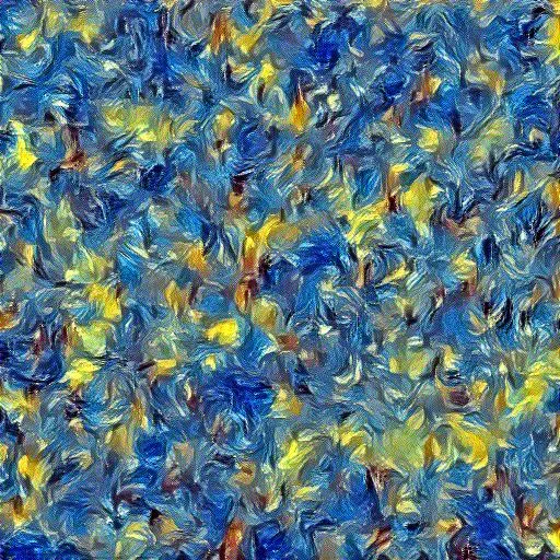
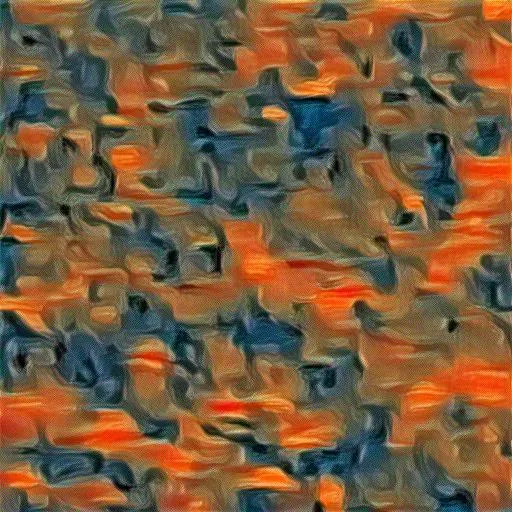
Below are some of the weird results.
I found there was no difference in runtime which was bizarre. I also think that my noise strength was too strong for noise intilization. If I had run them longer than 300 iterations maybe the content loss would’ve gone down but I’m very happy with the content intilization ones.
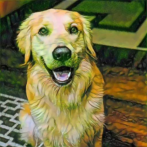
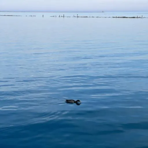
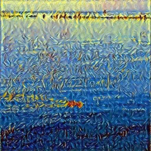
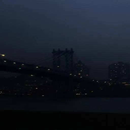
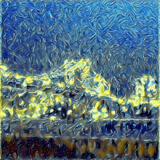
Finally there are some of my own images.
Bells & Whistles
Other Images
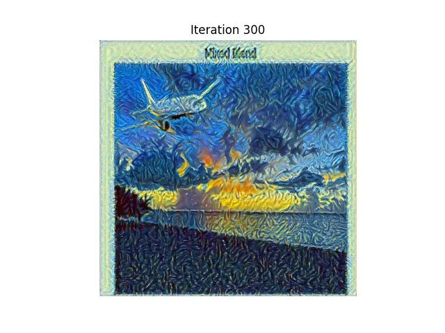
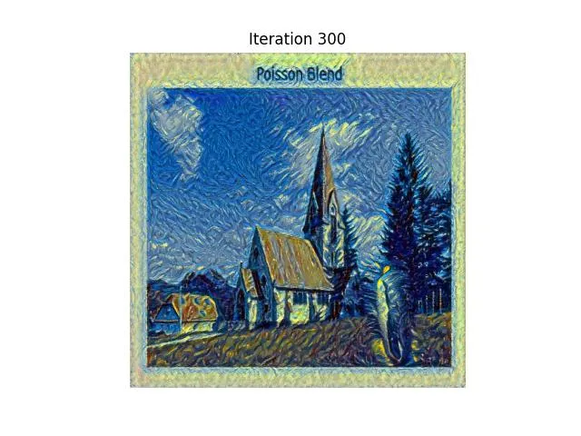
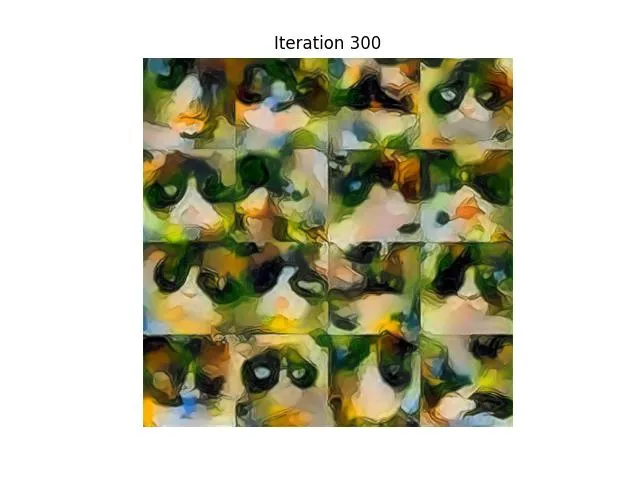
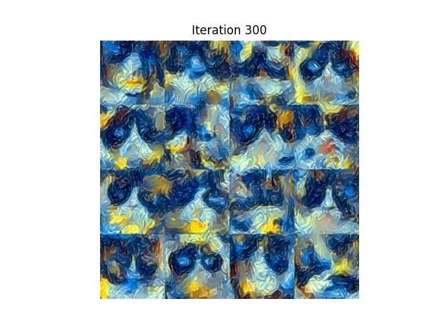
I also ran my style transfer on images from previous assignments. I did a poor job cropping the matplotlib edges and so we get to see stylized matplotlib templates. More papers should have stylized matplotlib templates.
Adversarial Learning
Recently I was listening to the following podcast on the show Oxide & Friends about Adversarial Machine Learning. They talked about how they optimize their images for a dual loss of desired adversarial behaviour while also not getting stopped by safety filters. In a classic classification vision context this would mean optimizing for a model to say that an image is an apple when really it’s a banana.
Anyways, I had the idea from this that instead of treating loss as strictly positive I could optimize for two different things. In general I ran experiments where I subtracted content loss from later layers from my base layer with the effect that hopefully the optimizer would lead to images that have high loss for deeper features. My initial experiments I thought were a failure until after playing around with the parameters I began to see Falling Water emerge. Below are my results as well as their parameters.
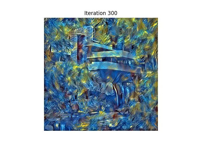
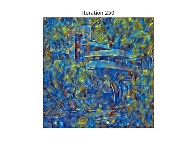
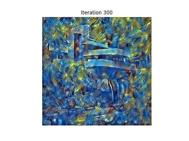
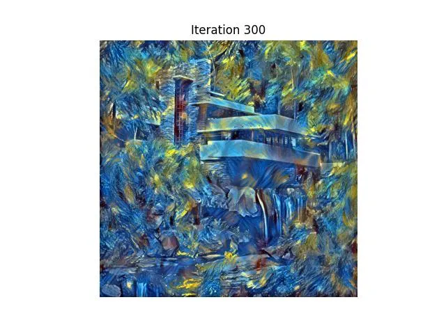
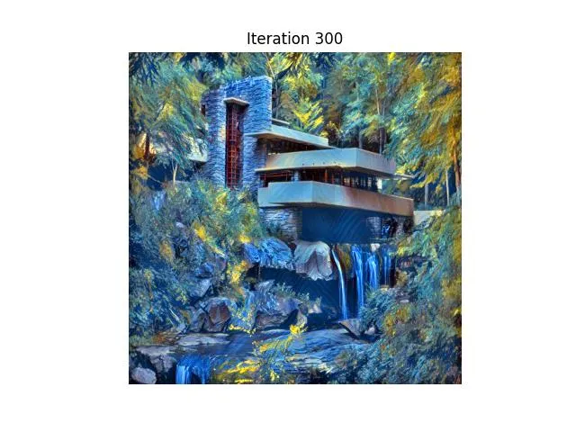
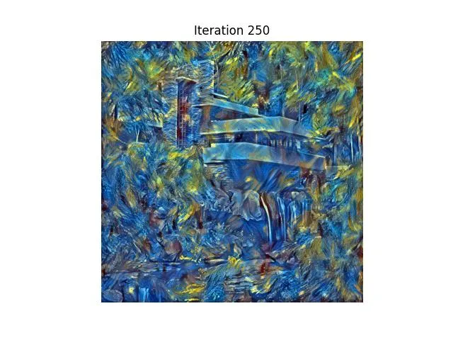
All results were initially using conv3 as our negative content layer. The nubmer then indicates the following experiments:
1 --> 0.00001 content_weight=100 style_weight =1000000
2 --> 0.0001 content_weight=100 style_weight =1000000
3 --> 0.0001 content_weight=100 style_weight =1000000  now using conv_2 as our base layer
4 --> conv1 as base layer and conv5 as negative layer
5 --> conv1 as base layer and conv4, conv5 as negative layer
While not perfect the results indicate that you can do interesting things like penalizing certain details while emphasizing others. For instance, there seems to be more style transfer on the borders letting the house remain.
Results
Appendix
All tests were run with the following fixed rand seed
RAND_SEED = 152
torch.manual_seed(RAND_SEED)
random.seed(RAND_SEED