Intro

Technical Difficulties

I had some technical difficulties with this assignment as it was not clear to me that when you request EC2 quota increases you should request vCPUs needed as opposed to number of instances. To get around this I converted the code to run on the M1 GPU if possible. Similar to CUDA a lot of my code had the following

if torch.cuda.is_available():
    G.cuda()
    D.cuda()
    print("Models moved to GPU.")
elif torch.device("mps"):
    mps_device = torch.device("mps")
    G.to(mps_device)
    D.to(mps_device)
    print("Models moved to M1 GPU.")

the main difficulty came with getting the dataloader to play nicely. No matter how I set my num_workers or parallel strategy I could not get the dataloader to execute with parallelsim. I finally settled on the following

def custom_collate(batch):
    batch = torch.stack(batch, 0)

    if torch.backends.mps.is_available():
        batch = batch.to(torch.device("mps"))
    return batc

dloader = DataLoader(
    dataset=dataset,
    batch_size=opts.batch_size,
    shuffle=True,
    num_workers=0 if torch.backends.mps.is_available() else opts.num_workers,
    collate_fn=custom_collate,

where the custom_collate handles sending the tensors to GPU memory. This could also be handled in the transformation passes but it’s messier as one needs to implement a custom transform.

Data Augmentation

To prevent overfitting of the discriminator we implement data augmentation that augments our real data. I chose to go with a random transform in my dataloader that was either

1. RandomHorizontalFlip
2. RandomCrop w/ Padding
3. RandomResize w/ CenterCrop

For 2,3 the additional operation was needed to make the tensors all the same size when they get put in GPU memory. With p=.8 one of these transformations were done but in retrospect I should’ve performed combinatorial operations to get more varied dataset from so few real images.

A more difficult dataset for the discriminator not only prevents overfitting but also most likely ‘slows’ its training which helps prevent the diminishing gradients when the discriminator and generator are in different stages of training, see Wasserstein Loss for more discussion of this.

Padding

In general we can calculate the new dimensions give input dimension, kernel dimensions, stride, padding using the following formula

Given that our kernel is,‘K=2’ and our stride is,‘S=2’ and we want our output to be half the size then we have the following for an arbitrary dimension

To solve that ‘p=1’ we need to case on parity of ‘i’. If ‘i’ is even then ‘p=1,0’ will get our desired outcome. If ‘i’ is odd then ‘p=1’ is the only soluton.

Therefore we take the intersection of possible results and get ‘p=1’.

We can see then for an arbitrary dimension our padding should be 1 with the given kernel and stride amounts.

For our first layer in our generator we don’t want to apply any upsampling we essentially want to

Results

Vanilla Gan

Basic Data Augmentation

w/ Diff Augmented

w/o Diff Augmented

Deluxe Data Augmentation

w/ Diff Augmented

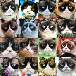
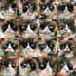
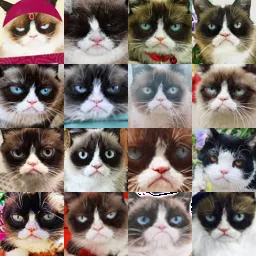
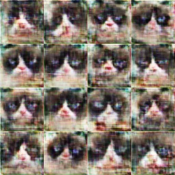
w/o Diff Augmented

Vanila Gan Discussion

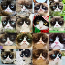
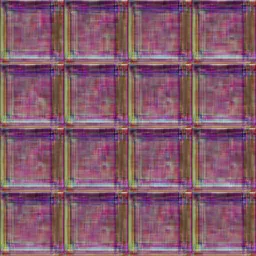
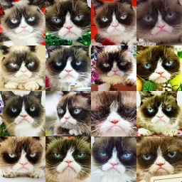
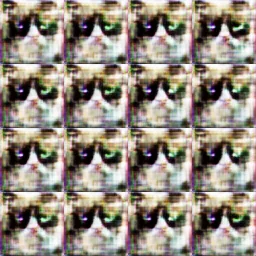
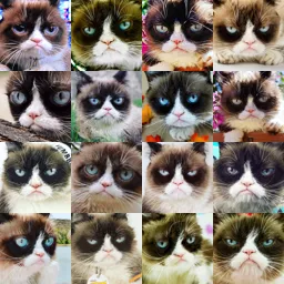
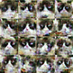
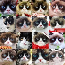
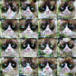
As can be seen from the results deluxe data preprocessing leads to more diversity in output. In addition, differentiable augmentation leads to better results with fewer artifacts.

In fact, the deluxe data augmentation is practically necessary as you can see in basic @ 3200 iterations there’s basically only noise. The deluxe data augmentation leads to faster convergence. This makes sense as it prevents the models from overfitting and creates more diverse data from a smaller dataset.

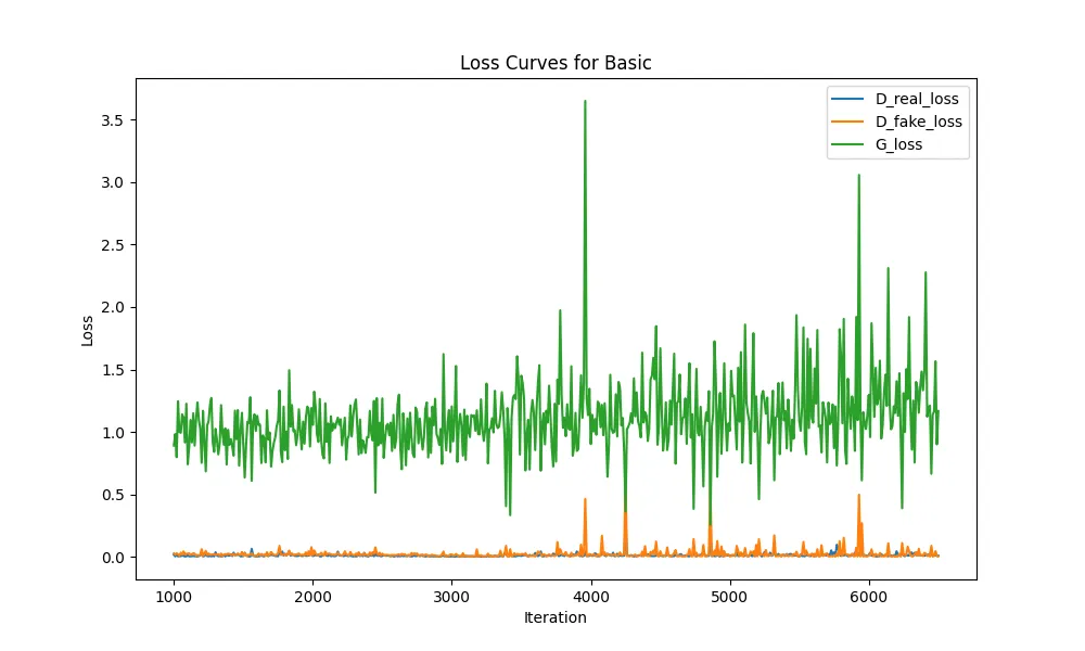
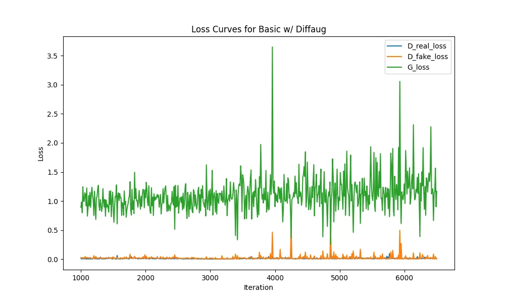
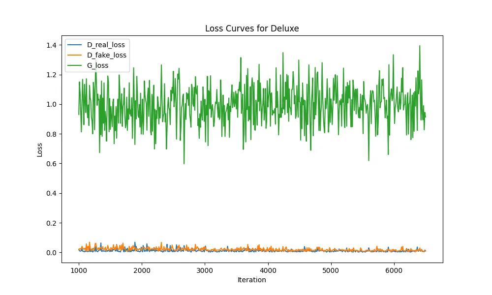
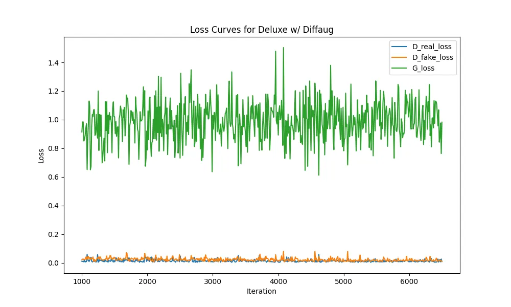
My loss plots are a little concerning as it seems my discriminators are too easily differentiating between real and fake imgages potentially leading to diminishing gradients. I could not get rid of this and I’m unsure why this was the case. As will be discussed later Wasserstein loss attempts to fix this.

Cycle Gan

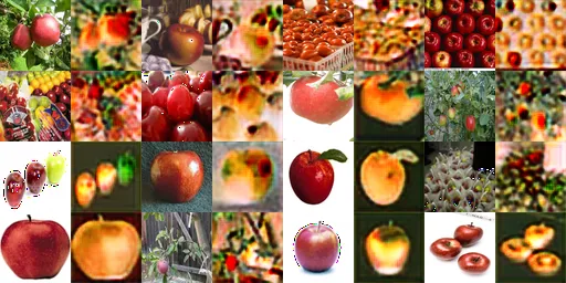
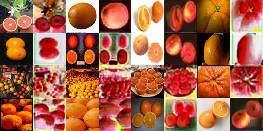
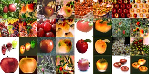
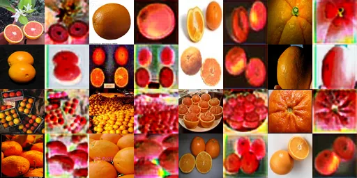
Apples2Oranges

DC Discriminator

w/ Cycleloss

w/o Cycleloss

Patch Discriminator

w/ Cycleloss

w/o Cycleloss

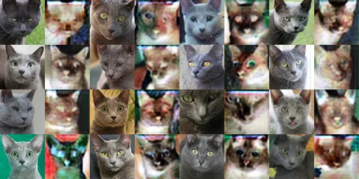
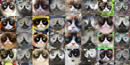
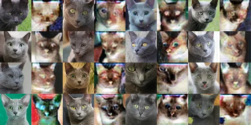
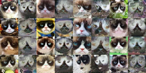
Cat2Cat

DC Discriminator

w/ Cycleloss

w/o Cycleloss

Patch Discriminator

w/ Cycleloss

w/o Cycleloss

Discussion

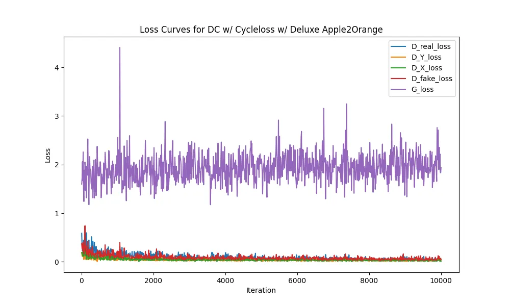
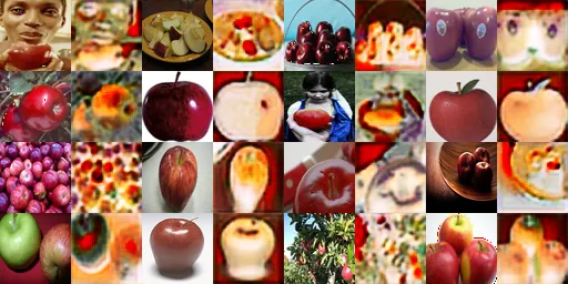
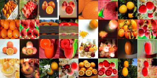
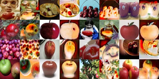
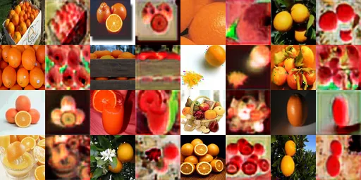
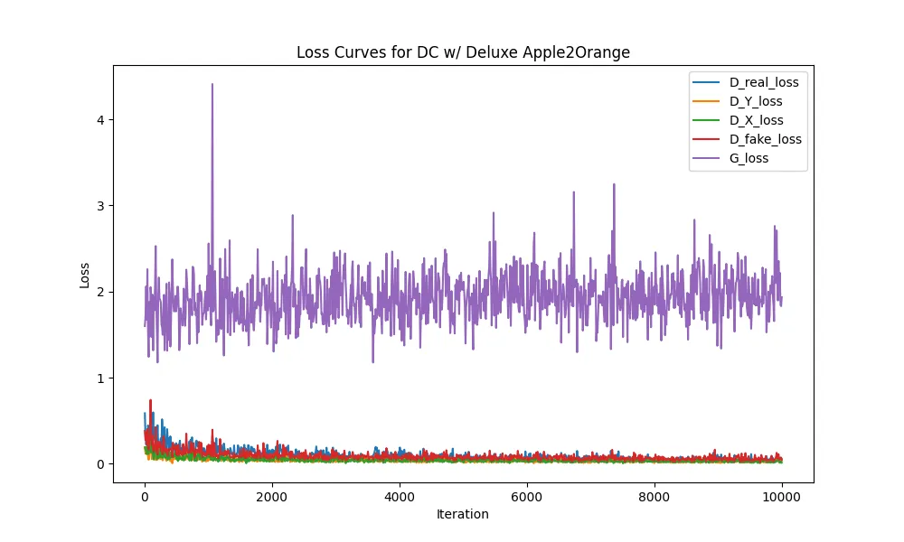
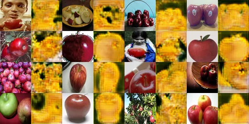
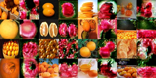
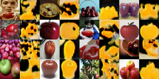
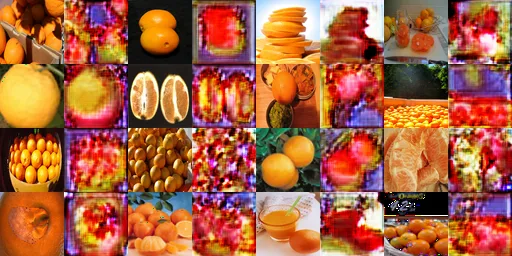
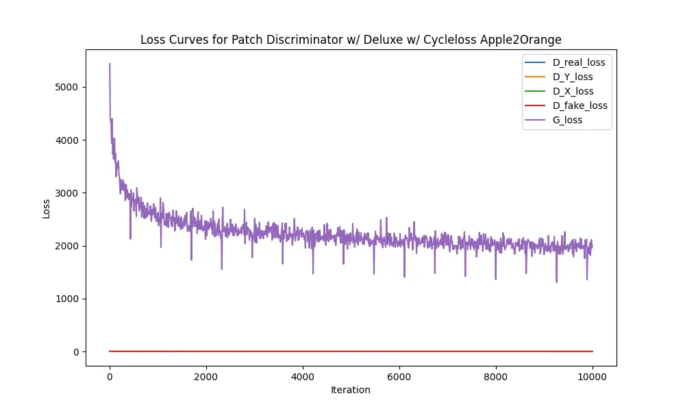
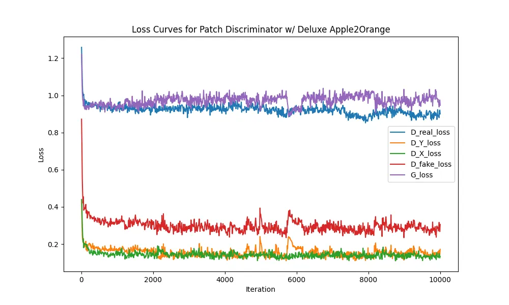
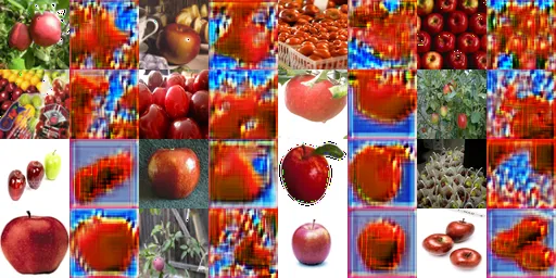
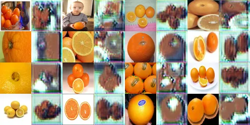
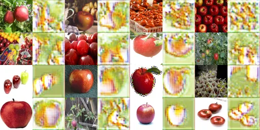
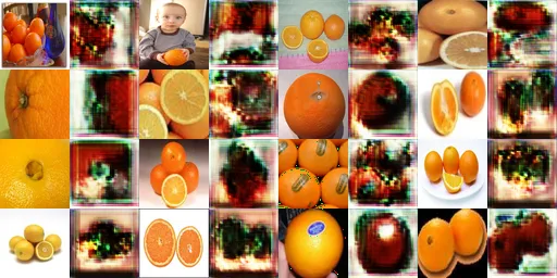
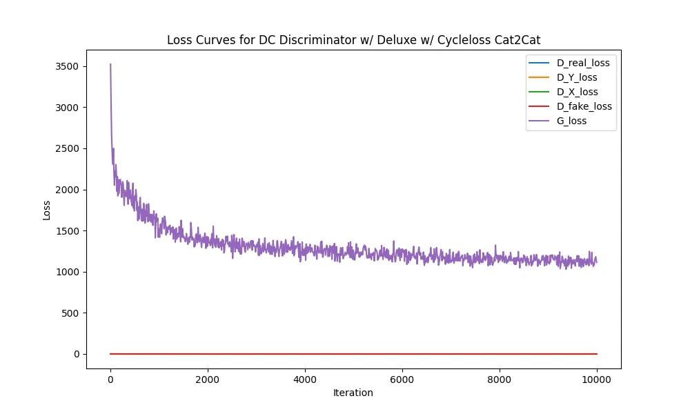
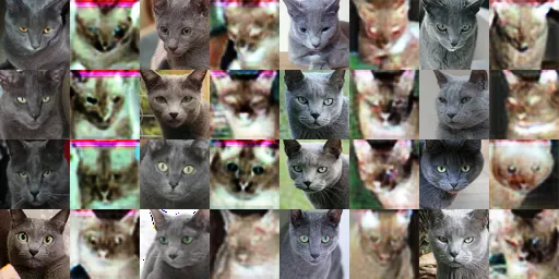
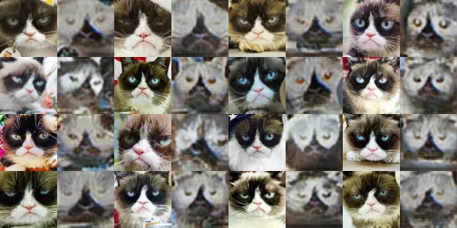
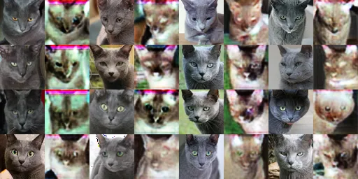
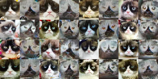
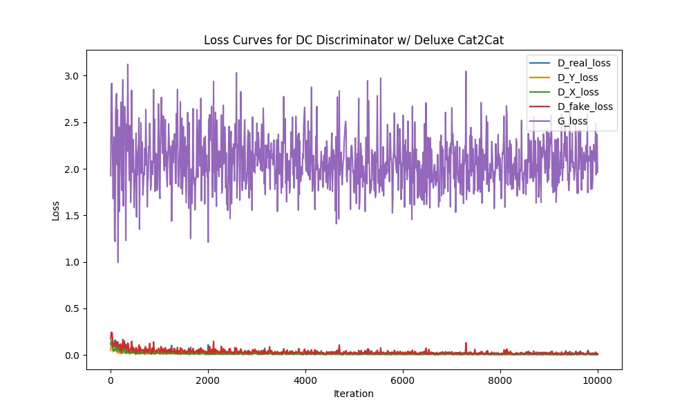
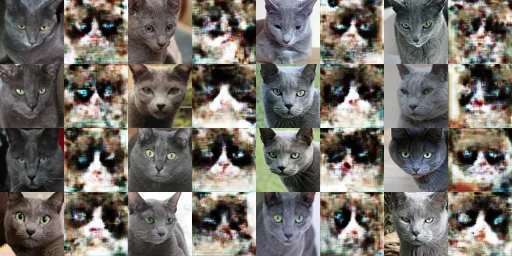
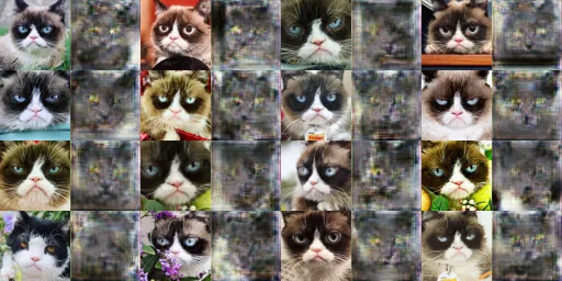
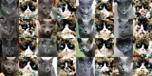
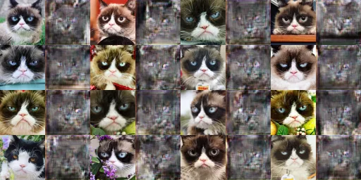
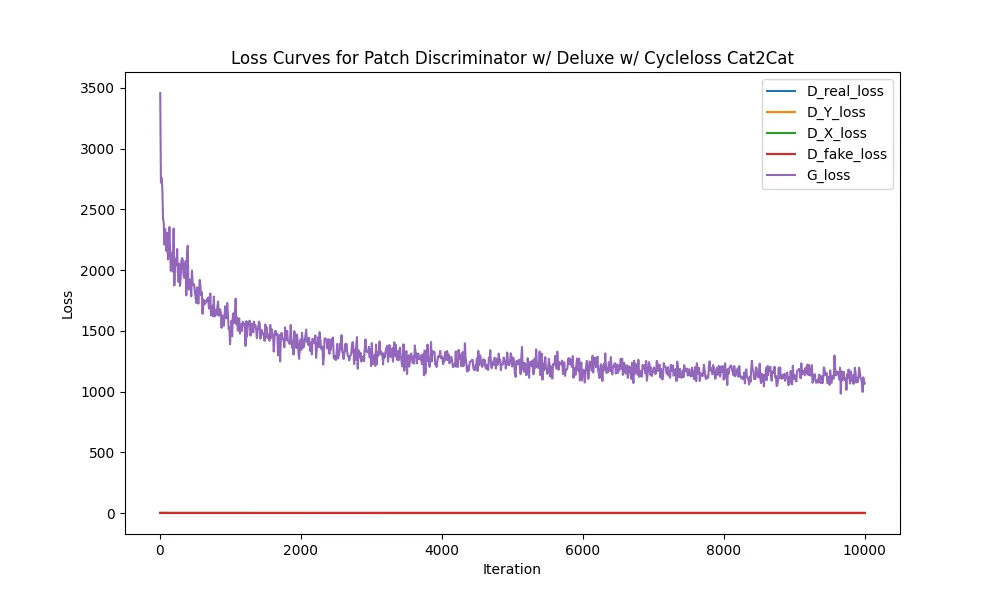
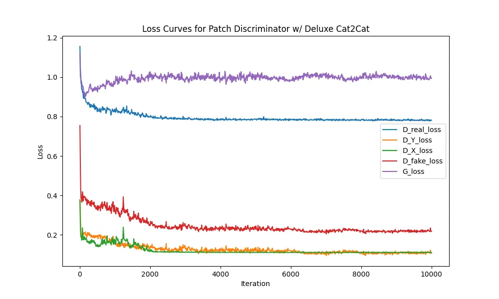
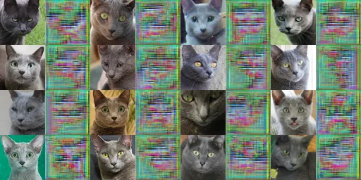
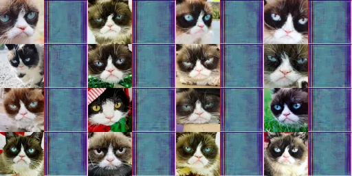
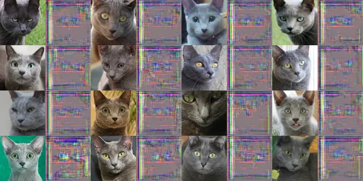
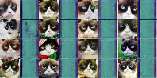
The results have not been cherry picked and there are instances of model collapse in the above images. While the losses overall look very bad the images aren’t terrible and if I had cherry picked the results I could’ve gotten better images. Without cycle consistency loss the models have a tendency to absolutely fall apart. This isn’t consistent behaviour, but cycle loss definitely helps prevent this. In addition, we can see cycleloss leads to better generator loss where it more monotonically decreases.

Another interesting result I found is that my Y->X results seem to be better than my X->Y. This is confusing as the code is symmetric for them but I think this is most apparent for the cats. It could be because the X cats are simpler than the black and white cats but I found these results confusing. In fact, as I look at some of the images, especially with the cats Y->X I get the impression that the output could be really good with slight color space changess. A similar thing happens in 10,000 iterations X->Y Patch Discrimnator w/Cycleloss. Some of the outputted cats are correct but others appear in the absolute wrong colorspace.

Overall, the patch discriminator performs better than the DC Discriminator as can be seen in Apples2Oranges where, even with Cycleloss Consistency, the DC Discriminator doesn’t display the Generator loss pattern that we’d like to see - decreasing and converging.

Bells & Whistles

Wasserstein Loss

A known issue with GANs is they’re notably unstable. For instance, if an optimal discriminator is achieved before the generator then the gradients for the generator dimish and the generator learns nothing. The origanl GAN paper suggests instead of calculating loss as

to instead do

However, our new loss function has remarkably high variance. One proposal to fix this is to add noise to generated images to stabilize the model. However, instead of adding noise we could instead use a new cost function - Wasserstein distance that has a smoother gradient everywhere.

The goal of WGANs is to learn no matter how the generator is performing. This circumnavigates the issue that it’s much easier, and probable, to develop a good discriminator versus a good generator.

The Wasserstein paper suggests using the Earth-Mover distance or Wasserstein-1 to measure divergence or loss

where $\prod (\mathbb{P}_r, \mathbb{P}_g)$ denotes teh set of all joint distributions $\gamma(x,y)$ whose marginals are respectively $\mathbb{P}_r, \mathbb{P}_g$ To translate it back into the nomenclature of EM-distance, $\gamma(x,y)$ indicates how much “mass” must be moved x to y in order to transform the distributions from one to the other, and the EM distance is the optimal cost of the transport plan. Note, inf is the infinimum.

However, the above formula is intractable, due to the infimum, therefore we use the Kantorovich-Rubinstein duality to get the following for our loss function

Where the supermum is taken over all 1-Lipschitz functions $f : \mathcal{X} \rightarrow \mathbb{R}$. In practice, this can be simplified to

which can then be approximated via backpropogation up to a mulitplicative constant.

We can represent this with the following psuedo code

for _ in range(n_critics):
    D_fake_loss = mean(D(fake_images))
    D_real_loss = mean(D(real_images))
    D_total_loss = D_fake_loss - D_real_loss

for parameters in D:
    # Enforce lipschitz constraint
    p.clamp(-0.01, 0.01)

G_loss = -mean(D(fake_images))

Note in the paper they update their discriminator multiple times per a step.

The clamping process is a working, albeit poor method, to enforce the Lipschitz constraint and force the weights to fit a fixed back thus enforcing $\mathcal{W}$ to be compact.

The hopeful end result is less instability during training.

Results

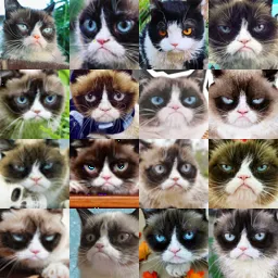
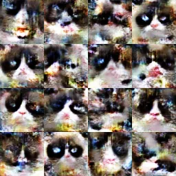
Note, in practice there is hyper parameter tuning controlling both the mixture of real and fake images during the discriminator training step, as well as normalization of the backprop. I chose to forego these which might be part of the reason the results are the way they are.

Discussion

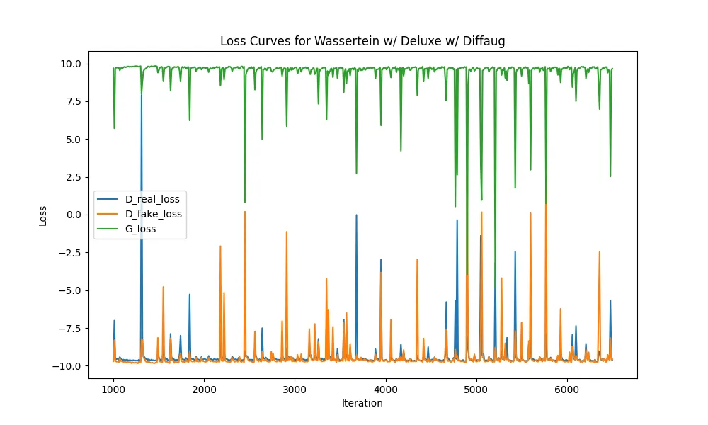
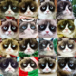
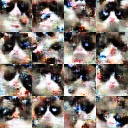
The Wasserstein loss graph doesn’t look great but it’s hard to say what part of this is inherent to GANs. I will say the results actually look quite good despite the artificating. I’m sure with further hyperparameter tuning as well as doing the mix of critics I could’ve improved the results.