Explanation

This project explores gradient-domain processing a technique that uses gradients to better blend images together. We start off with a toy problem recovering an image from x,y gradients and then move on to poisson blending.

Our main goal throughout this assignment is to solve for

v = \argmin_{v} \sum_{i \in S, j \in N_i \cap S} ((v_i - v_j) - (s_i - s_j))^2 + \sum_{i\in S, j \in N_i \cap \neg S}((v_i - t_j) - (s_i - s_j))^2

where $s_x$ represents pixels in our source image, $t_x$ represents pixels in our target image, and $N_i$ represents our mask (this is an oversimplification we’ll correct later).

In essence we want to find $v_i - v_j$ , a new gradient, such that it’s L2 loss compared to the gradient of our source image is minimized. We do this by constructing the matrices $A,b$ and using a least squares solver to find $v$ such that $Av=b$ .

Note our matrices were fairly sparse so throughout we use sparses matrices to speed up computation.

I found this assignment somewhat frustrating because the results could either be really good or really bad. When they were really bad I went through all my code looking for errors only to realize this method, as implemented, can be incredibly brittle.

Toy Problem

Our toy problem introduces us to gradient processing and asks us to reconstruct an image from its gradients.

Using s(x,y) to denote intensities at (x,y) and v(x,y) to denote the pixels we want to solve for we come up with the following three equations.

Minimize $((v(x+1,y) - v(x,y)) - (s(x+1,y) - s(x,y)))^2$ ie the x-gradients should match
Minimize $((v(x,y+1) - v(x,y)) - (s(x,y+1) - s(x,y)))^2$ ie the y-gradients should match
Minimize $(v(1,1), - s(1,1))^2$ the top left corner should match exactly (this is essentially assignment).

In code this looks like the following for the x-gradient:

A[..., im2var[y, x + 1]] = 1 
A[..., im2var[y, x]] = -1
b[...] = s[y, x + 1] - s[y, x] # x-gradient at y,x

We are solving for the corresponding v_i, v_j such that (v_i - v_j) - (s[y,x+1] - s[y,x]) is minimized. im2var can be thought of as mapping coordinates to variables.

Our results are below:

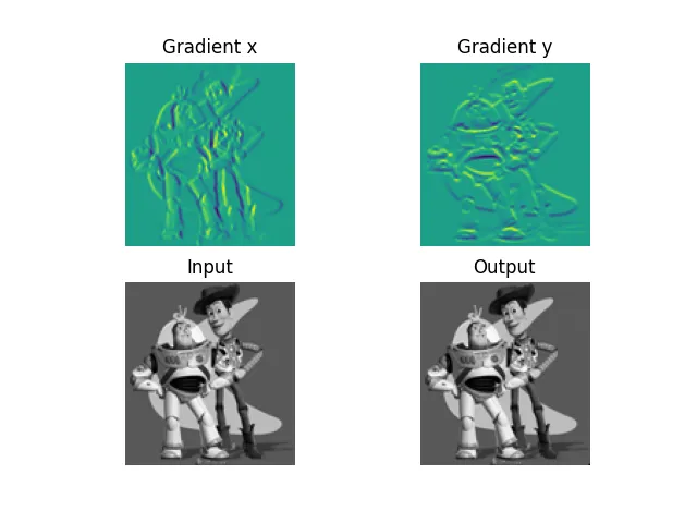
ToyProblem. With L2 difference of .348 we’ve almost perfectly reconstructed the input.

Poisson Blending

For the main part of the assignment we want to solve a similar equation as above but with some more steps. We’ll use the terminology source to refer to the image that’s getting blended in, target to be the background that’s getting blended onto, and then mask to refer to a mask over our source.

v = \argmin_{v} \sum_{i \in S, j \in N_i \cap S} ((v_i - v_j) - (s_i - s_j))^2 + \sum_{i\in S, j \in N_i \cap \neg S}((v_i - t_j) - (s_i - s_j))^2

While this equation can seem intimidating we’ll break it down.

$i\in S, s_i, s_j$ covers pixels in our ‘source’ image and within our mask. Here we want the new solved pixels to have a small gradient. j is the 4 pixels above, below, to the left, and to the right of our target pixel v_i.
If we are outside our mask ie $i \in N_i \cap \neg S_i$ then we are dealing with pixels on the border of our mask. In this case we want to minimize (v_i - t_j) - (s_i - s_j) where t_j is not from our source but our target image. The idea being we want a smooth transition to the background image and thus want to minimize our edge gradient.

As in the toy example we build sparse matrices and then use scipy.lsqr to solve them.

Results

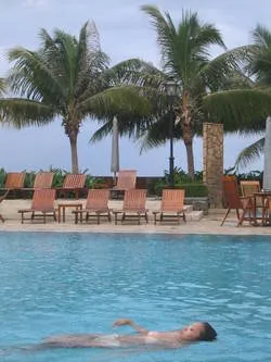
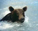
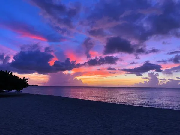
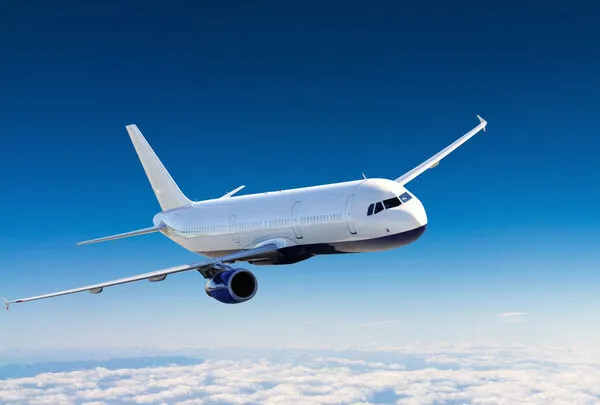
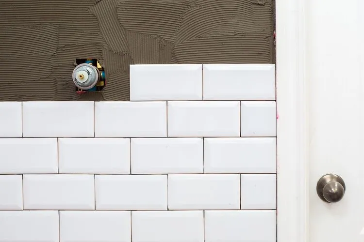
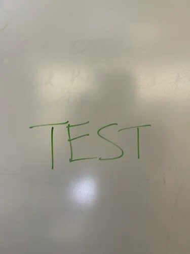
First we present some our source materials. The first column is the target and the other columns are various sources.

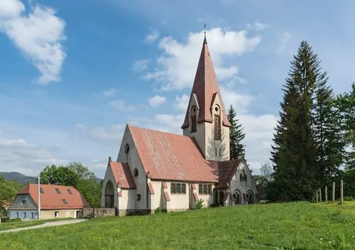
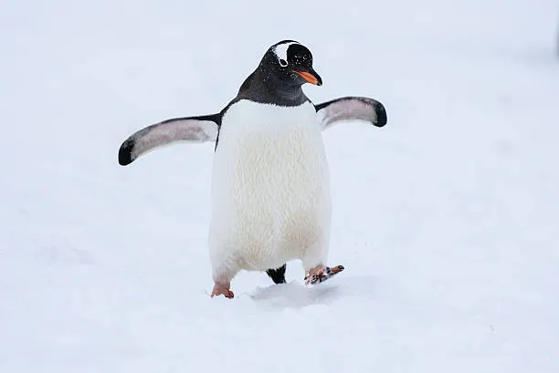
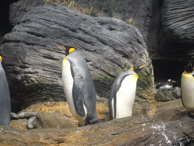
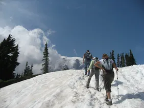
Now we show our results.

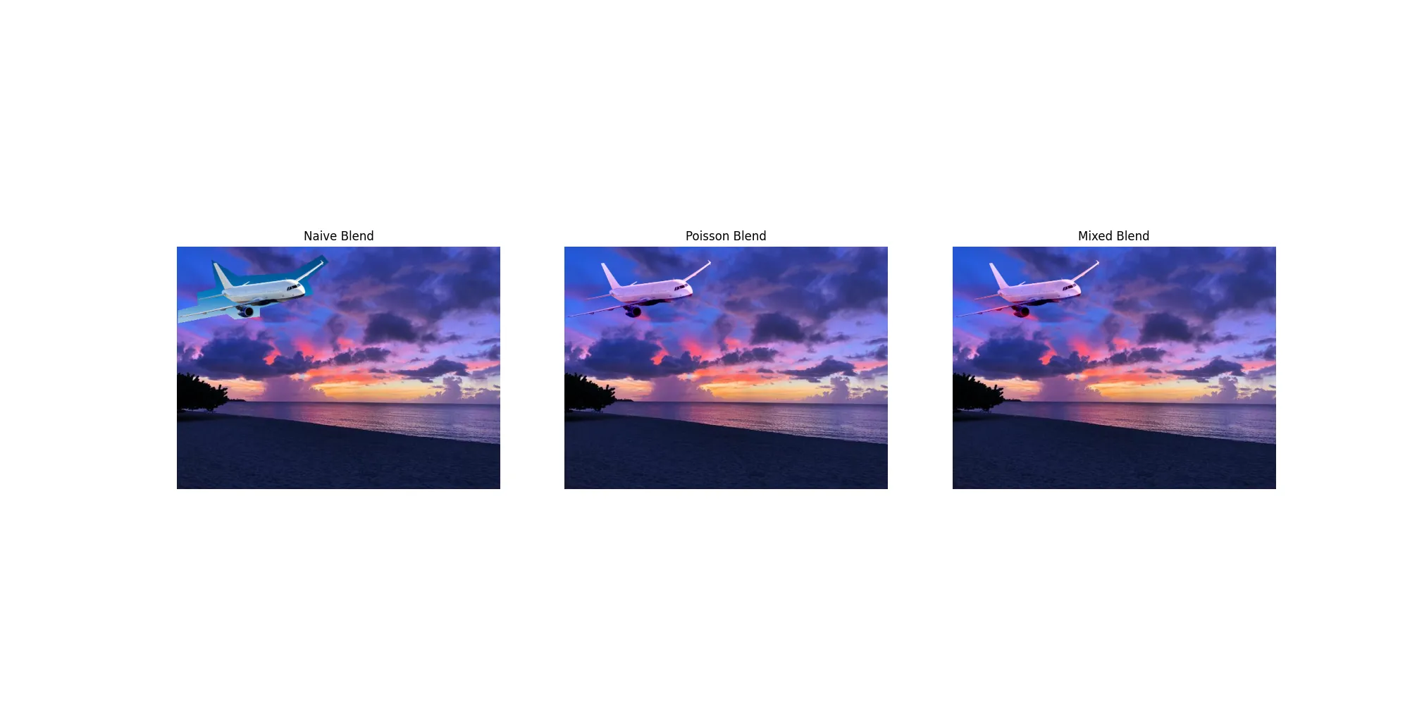
Plane with a nice sunset

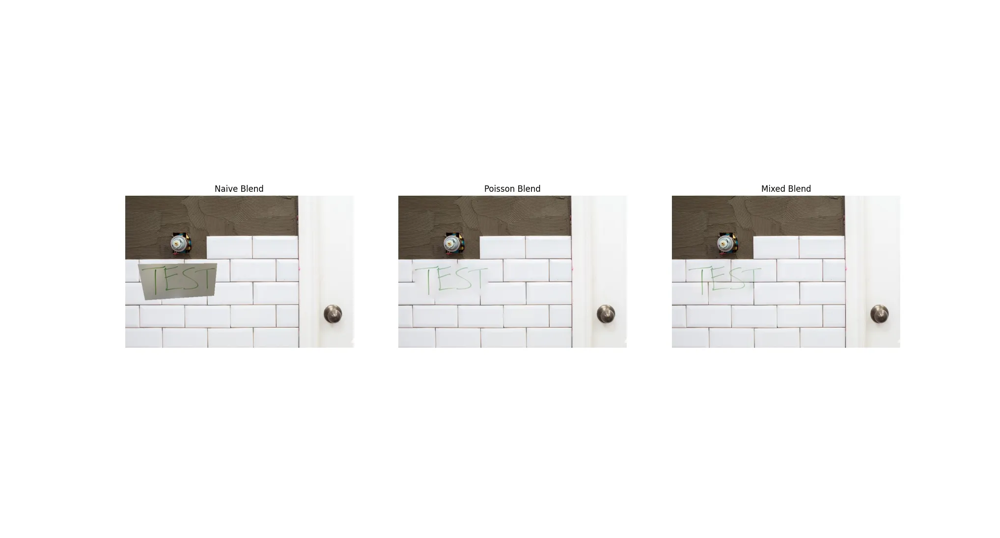
Writing on tile. Notice how with mixed blending the underlying grout shows through. Exactly what we want.

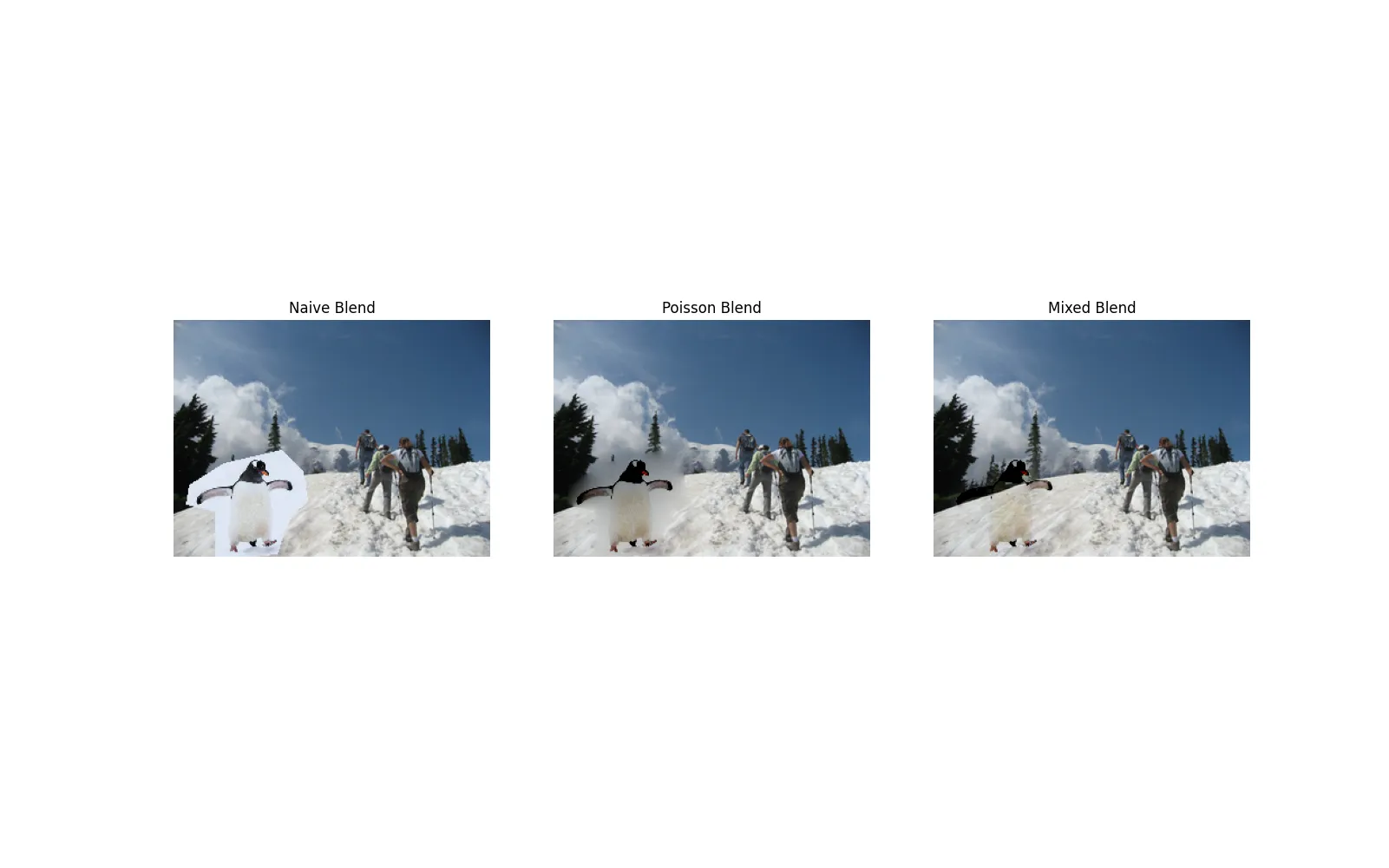
A penguin with skiers. Note how with the bad mask we get lots of blurring with poisson blending and with mixed blending the background bleeds through the penguin.

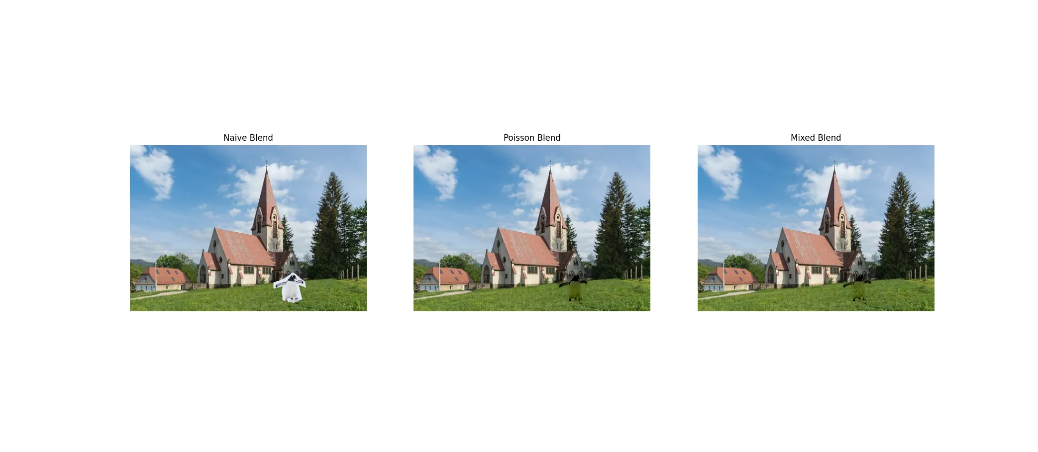
More penguins on a field. Once again these results aren’t great. The dark grass makes the penguin much darker than it needs to be and with mixed blending we’ve lost the body of the penguin! This makes sense as the gradient across a solid white surface is going to be zero compared to the texture grass below.

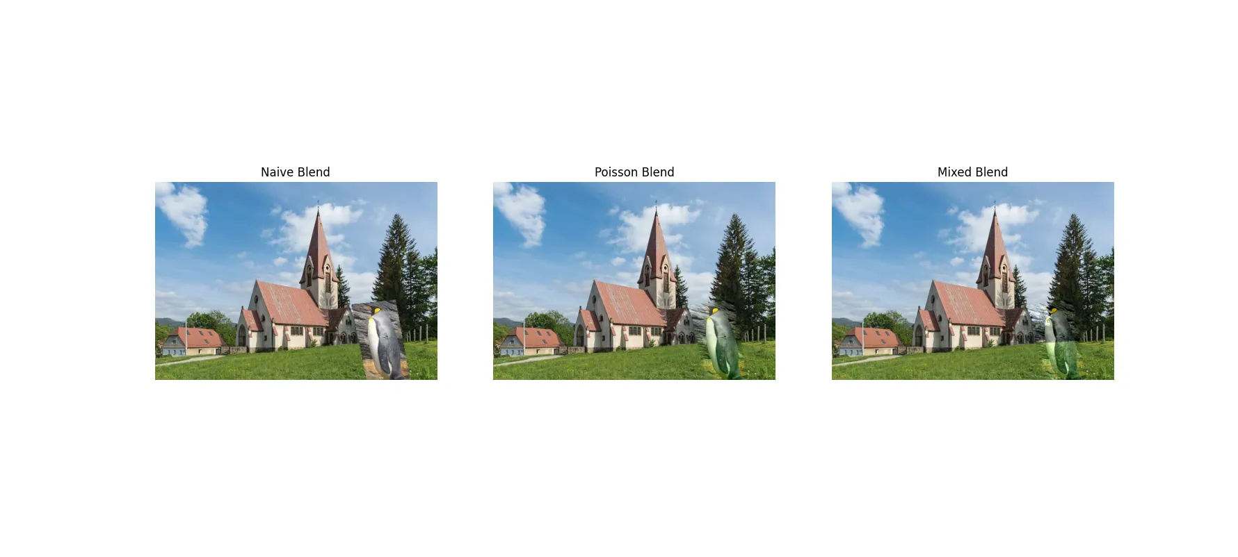
Even more bad penguins! Here the background of the penguin that got included in the mask was very complicated leading to bad results. The penguin also developed an undesirable green cast because it’s overlayed over grass. Generally this technique comes out better when you have solid monotone backgrounds as they blend more easily.

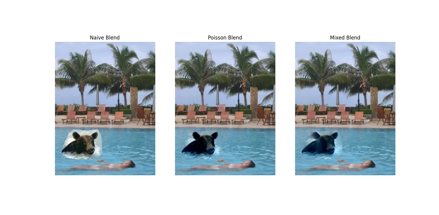
Swimmer with bear. Look out!

Bells & Whistles

Mixed Gradients

We now want to minimize the following

v = \argmin_{v} \sum_{i \in S, j \in N_i \cap S} ((v_i - v_j) - d_ij)^2 + \sum_{i\in S, j \in N_i \cap \neg S}((v_i - t_j) - d_ij)^2

where $d_{ij}$ is defined as

if abs(s_i - s_j) >= abs (t_i - t_j):
    d_ij = s_i - s_j
else:
    d_ij = t_i - t_j

The results for mixed gradients are displayed above. Because the strongest gradient is allowed through there were weird results where the background would bleed through the target. This was desired when the target was handwriting and we wanted to preserve the tile underneath but was less desired with the penguin on the grass. One interesting result I found is that with a bad mask this strategy led to much better results. With poisson blending a bad mask could leading to weird blur which this method avoided. This is probably because a bad mask let in more background than it needed and the backgrounds had smaller derivatives that got ignored leading to better blending even with a bad mask. You can see this with the various penguins, even though the background bled through the chest of the penguin the edge’s, where the bad masking is, look really good. Perhaps a dual strategy could be employed to get the best of both worlds.

color2Gray

This was a disappointing experiment as, it should’ve worked but failed miserably. The main idea is we convert the image to gray naively and then we find the number and find the layer with the greatest contrast in the HSV color space and then use the number as a mask to pertube the values in the naive conversion. This way we can make the resulting image contrastier without deviating too much from a grayscale image and still maintaining the key contrast of the colored image. V was used as it often maintained the contrast of the original image.

I spent way too much time on my automasking code only to realize my results weren’t as strong as I would’ve liked them. My automasking strategy was in the H layer I created 3 bins with $\mu \pm \{\sigma, 0\}$ and then autobinned pixels and took the upper most bin or lowest bin indices to form my mask. This strategy was developed as I noticed in H there would be a strong positive or negative (ie lack of) activation where the numbers were. This strategy worked great for samples like 74, or 6, but failed other times.

Results

As mentioned my results leave a lot to be desired, either the mask failed or the resulting image wasn’t pertrubed as much as I would’ve liked.

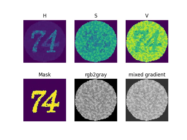
Ishihara 74, V isn’t that contrasty so the results don’t get pertrubed in a noticeable way

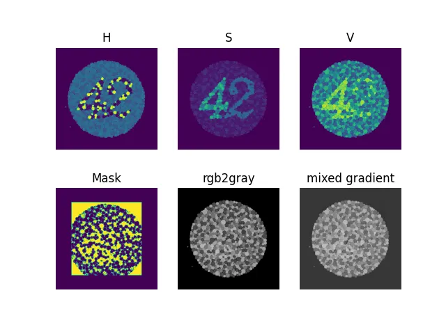
Ishihara 42, the auto mask failed, we can see H doesn’t have an obvious way to partition it.

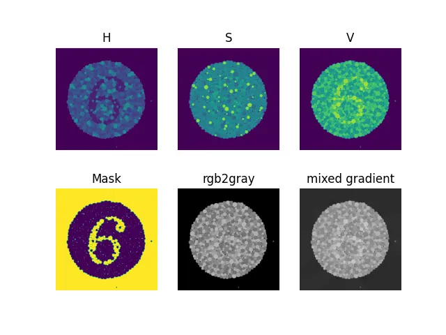
Ishihara 6 - this worked!

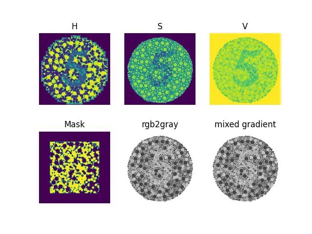
Ishihara 5 - we chose the wrong bins and hence our mask is really bad.

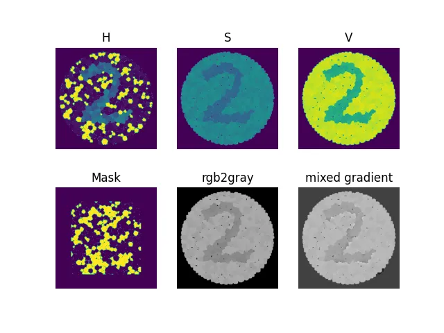
Ishihara 2

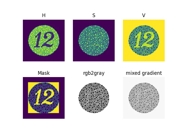
Ishihara 12. This one actually worked but Matplotlib’s c2gray is doing some weird tone mapping making it not seem apparent.

Original Ishihara colorblind tests

Conclusion

As I said I struggled more than I should have with this assignment as I often thought my code wasn’t working when really it was just brittle. The concept of gradient domain processing is very powerful but to get it to work across a variety of workloads would require a lot more finetuning and analysis.