Brief Description

Image taken from https://commons.wikimedia.org/wiki/File:Gradient_descent.gif

Image taken from Google

This project is aimed at utilizing a technique called gradient-domain processing. For this homework we are asked to place an image and integrate it with another one. We aim to make this transition look real. One method of doing this is directly copying and pasting pixels from the source image to the target image. The problem with this is that it can be quite obvious that these are 2 images put on top of each other, therefore we take advantage of using gradients. We want a smooth transition and blend to make the image look more realistic, and this is the objective of this assignment.

Toy Problem

For the toy problem, we try to simplify Poisson Blending. Instead of looking at all 4 directions , we focus on looking at the neighboring pixels directly above and below the pixel. We will also look at the first pixel of the image to help us with reconstruction.

Calculating gradients

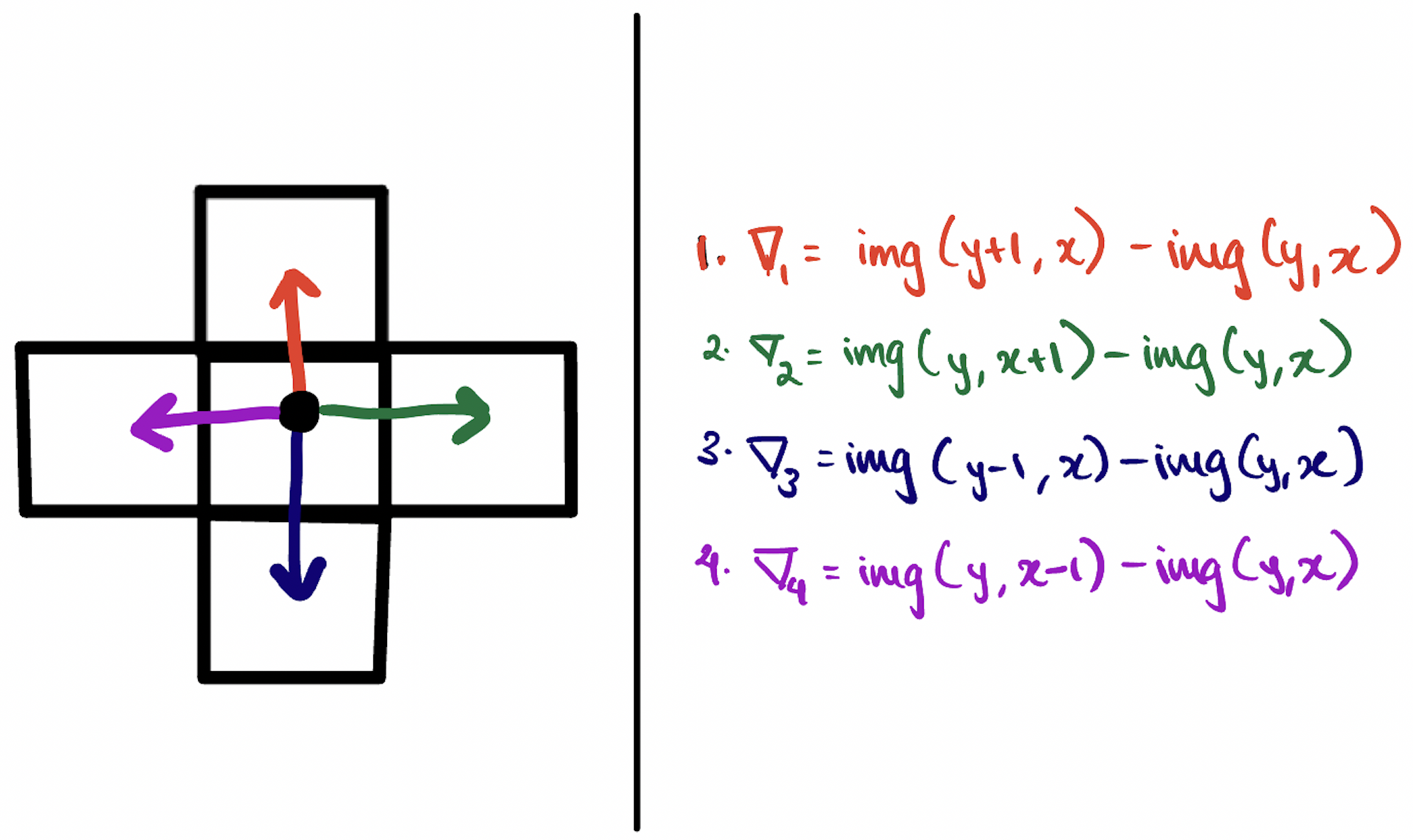
In order to solve this problem, we need to minimize the following objectives:

((v(x+1,y)−v(x,y))−(s(x+1,y)−s(x,y)))²

((v(x,y+1)−v(x,y))−(s(x,y+1)−s(x,y)))²

(v(1,1)−s(1,1))²

This can be turned into a least squares problem. We use matrix A to hold the coefficients of our system of linear equations. We create an equation for every pixel in the image and every direction of gradient we're taking, as well as one extra equation for the leftmost pixel that matches the rightmost pixel. This means for this particular toy problem, we should have (2 * height of image * width of image) + 1 number of equations. The number of places in a row is (height of image * width of image) because we are flattening our image into a 1D array for our system of equations to work. We use these equations to calculate the gradient of a pixel in a particular direction. While we iterate through all the pixels to create our matrix A, we need to also construct our matrix b which contains our desired target values. The essence of our algorithm lies in attempting to get the gradients of the target image to match the gradients of the source image as much as possible. So for our values in b that involve gradients, we take the gradient of the respective pixel in the source image. For the last equation that observed the leftmost first pixel, we keep our respective value in b as the source image pixel intensity itself. Then we use these matrices to solve for vector v that will contain our target image's pixels.

In the code implementation, we use sparse matrices as computation on a normal matrix for a large number of pixels can take a very long time. First scipy's csc_matrix was used because there was a SparseEfficiencyWarning that mentioned "Changing the sparsity structure of a scs_matrix is expensive". The toy problem took 25.06 seconds to run using csc_matrix, but only 3.54 seconds to run using lil_matrix. Hence, we proceeded to use lil_matrix to initialize the sparse structure. Function scipy.sparse.linalg.lsqr was used to solve our equation.

Poisson Blending

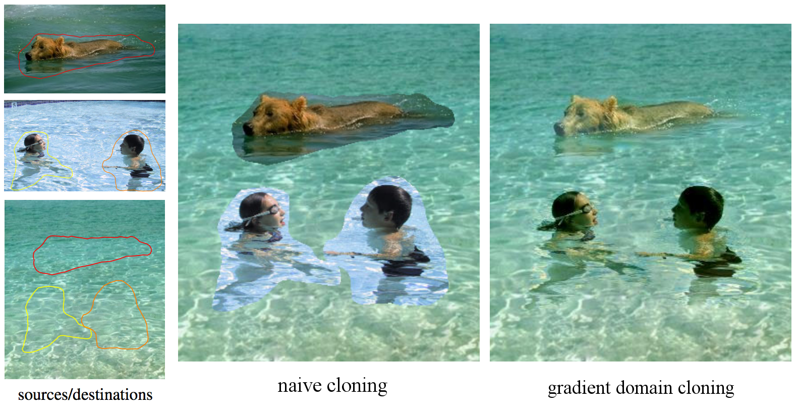
Following the explanation of the toy problem, now we expand our solution to apply Poisson blending. This means now we are looking at all 4 directions to observe neighboring pixels and gradients. I referred to https://cs.brown.edu/courses/cs129/results/proj2/taox/ to help formulate this.

Here this becomes the equation we wish to solve:

The two summations can be divided into 2 different tasks i.e the first term indicates that if the pixel AND neighboring pixel are inside our mask, then we keep b[e] as (s_i - s_j). If the neighboring pixel is not part of the mask then b[e] is (s_i - s_j + t_j) [where s is source image and t is target image]. The pixels outside of the mask, we keep the same. Once we have constructed our matrices, we once again solve them to find the least squares solution.

Results

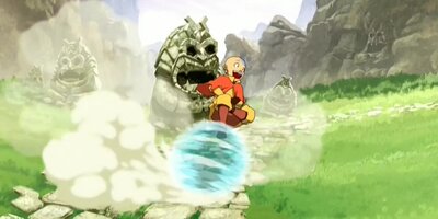
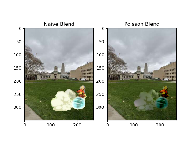
My favorite result would be the following just because I am a huge Avatar The Last Airbender fan and wish he could come to campus. The result isn't the best because Aang should ideally be more opaque, but I still like this image. Better results will come later.

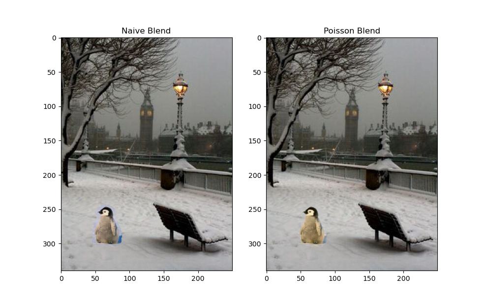
Here we keep a small penguin near the Big Ben in London. As we can see, the Poisson Blended image looks more realistic than the naive approach.

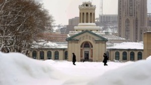
Now we try to implement our method to recreate the popular Bernie Sanders inauguration meme from 2021.

Here is an example of a bad result...

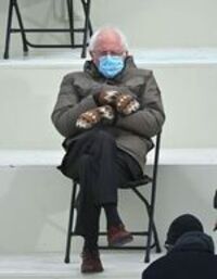
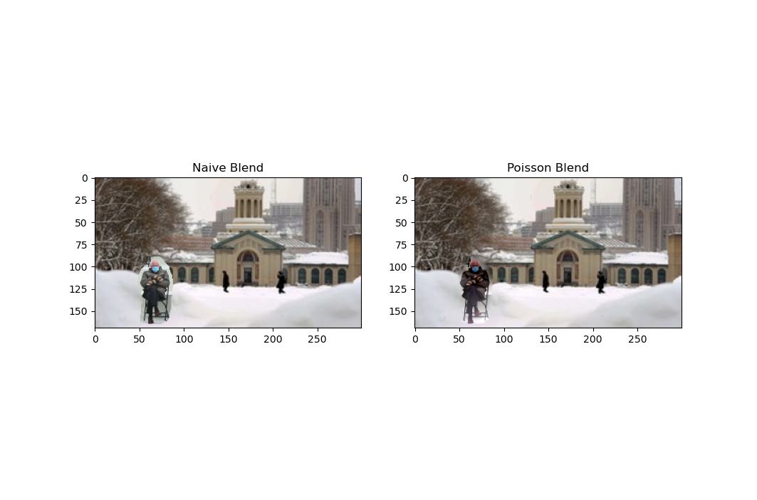
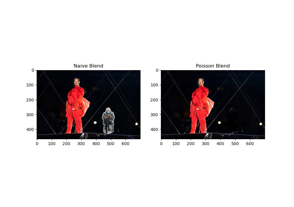
As we can see here, Bernie Sanders has disappeared :(

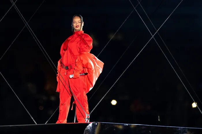
This is likely because the majority of Rihanna's image is the stadium which is dark because she is in the spotlight. So blending Bernie into Rihanna's image involves trying to blend very different pixel intensities where the stadium behind her have pixel intensities close or equal to 0. It becomes difficult to see Bernie because his image is now heavily influenced by the pixel intensities of Rihanna's. That's why when applying Poisson blending, it is advisable to choose images that have similar histograms of pixel intensities and RGB values.

Bells and Whistles

Mixed Gradients

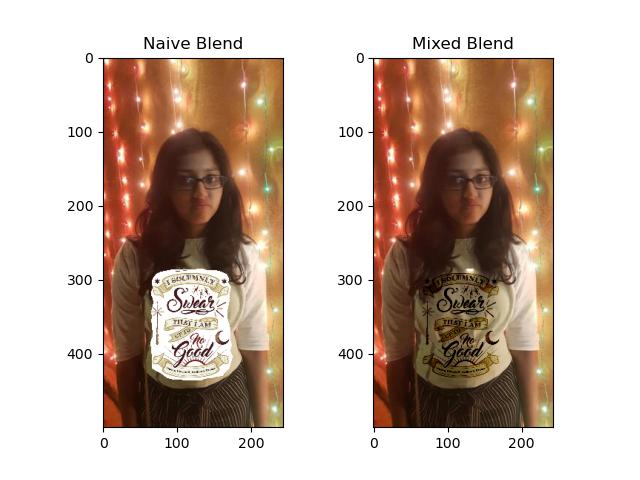
For using mixed gradients, we make a slight change to our algorithm in Poisson blending. Here this becomes the equation we wish to solve:

Our d_ij is dependent on the magnitudes of the source and target gradients. If the magnitude or absolute value of the source gradient is larger than or equal to the target gradient, then d_ij is the value of the source gradient (note that d_ij becomes the value of the source gradient, NOT the magnitude of the source gradient). Otherwise, d_ij is the value of the target gradient.

This change in the algorithm allows us to give a more transparent look, making it easier to do things like adding writing to new surfaces.

Results

My friend and roommate Shivani loves Harry Potter. Unfortunately I have a bad habit of giving birthday presents late. I've been meaning to gift her a nice Harry Potter shirt, but I dedicate this assignment as a temporary gift to her instead.

Color2Gray

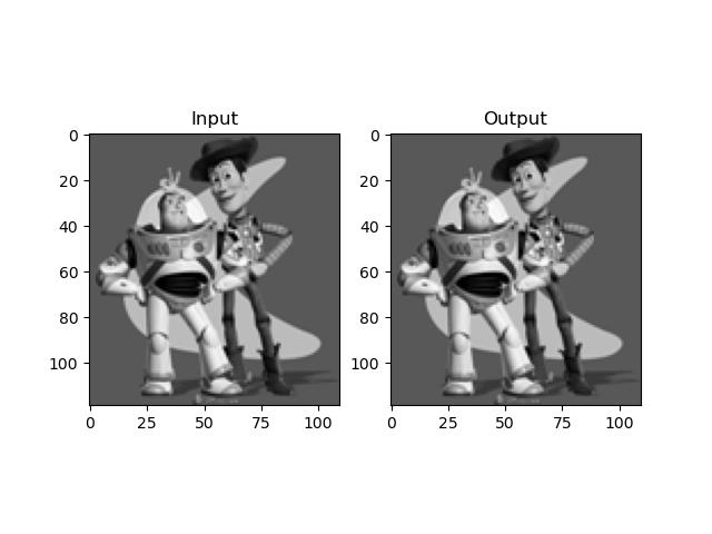
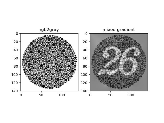
For Color2Gray, we see that often when we convert color images to grayscale, the contrasts between different pixels can be lost. With gradient domain processing, we can attempt to preserve this contrast information. The HSV color space contains information about hue, saturation, and value. We utilize the saturation and value channels of our image after converting it to the HSV space. I kept the saturation channel as the source image and value channel as target image to preserve the contrast information. The results are shown below:

Results

Other: Non-Photorealistic Rendering

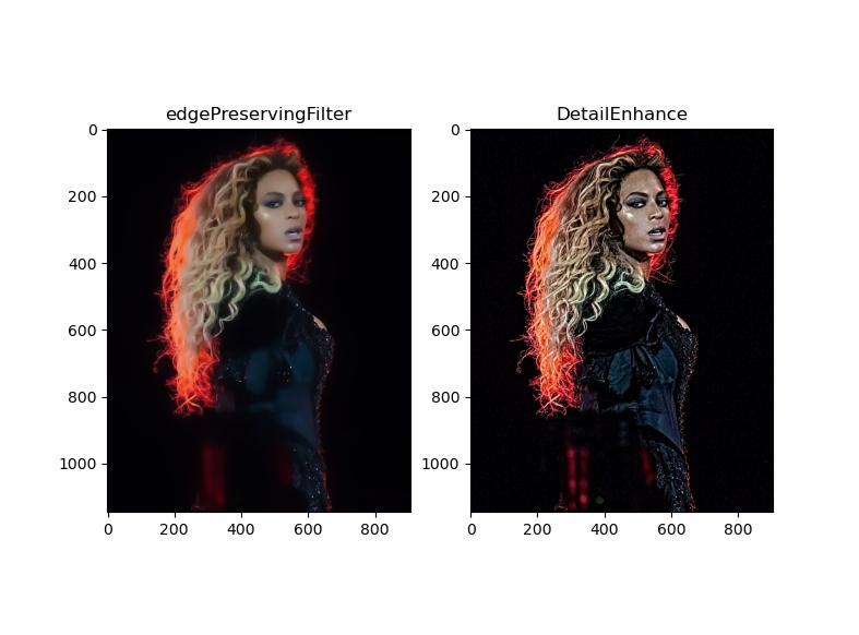
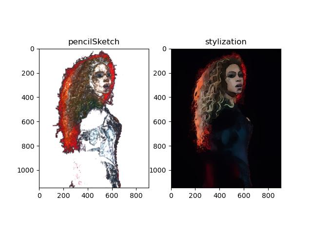
OpenCV has a lot of interesting functions that perform non-photorealistic rendering such as edgePreservingFilter,detailEnhance,pencilSketch, and stylization. I am a huge Beyonce' fan (she's coming to Pittsburgh!) so I used her picture for fun.

Here are the results: