Cathedral.jpg
Offset[R]: (12,3)
Offset[G]: (5,2)
|
Cathedral.jpg
Offset[R]: (12,3)
Offset[G]: (5,2)
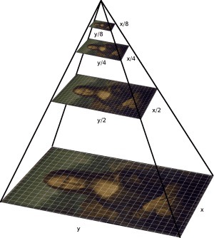
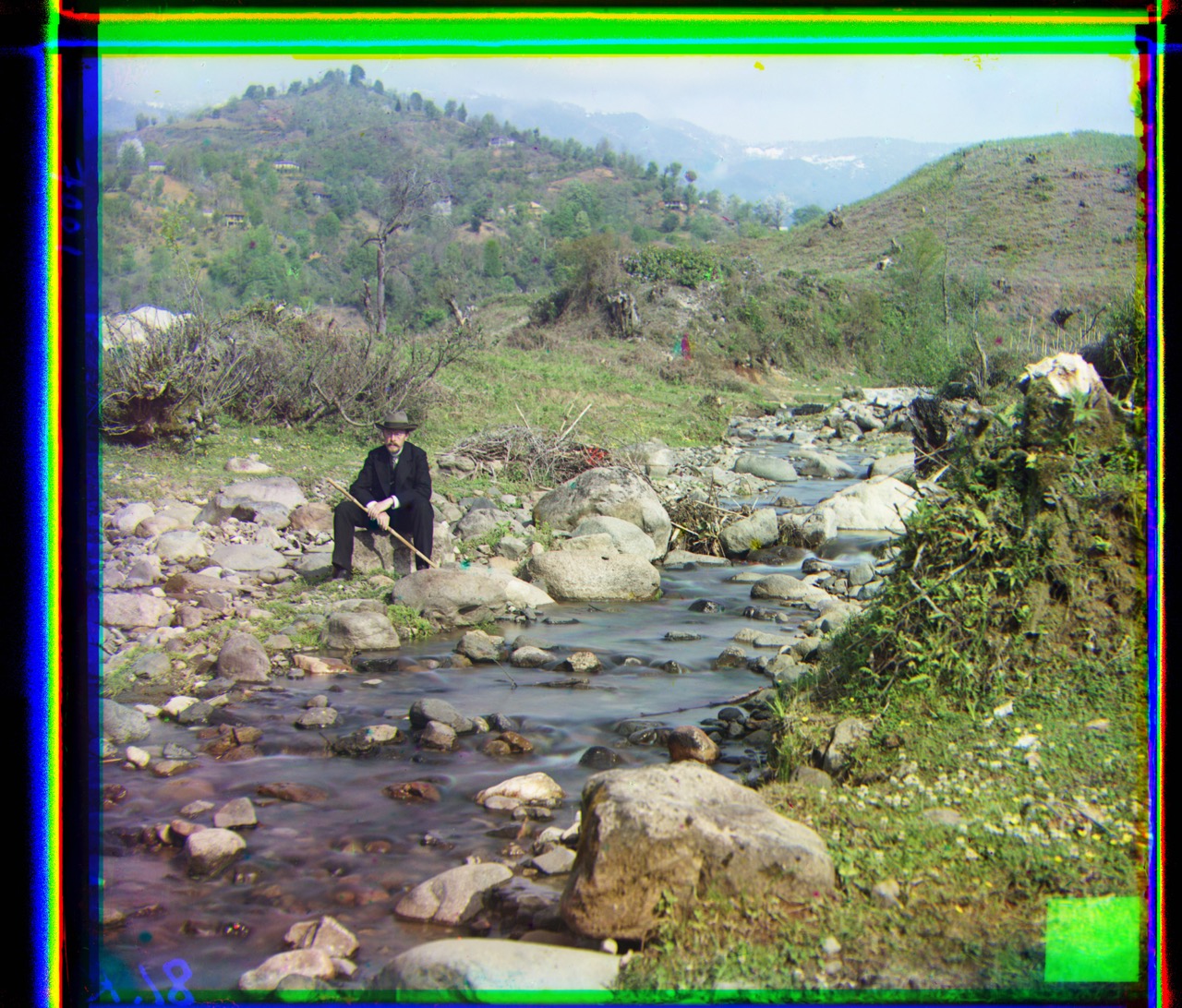
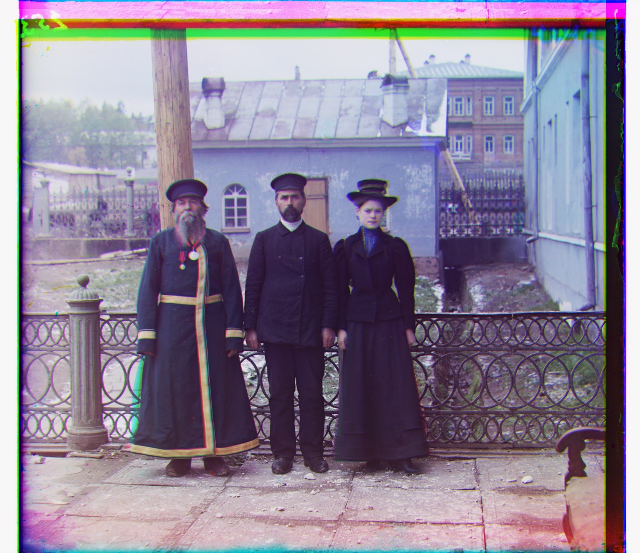
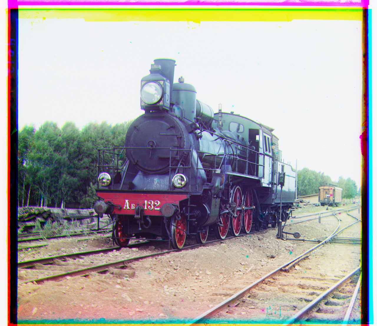
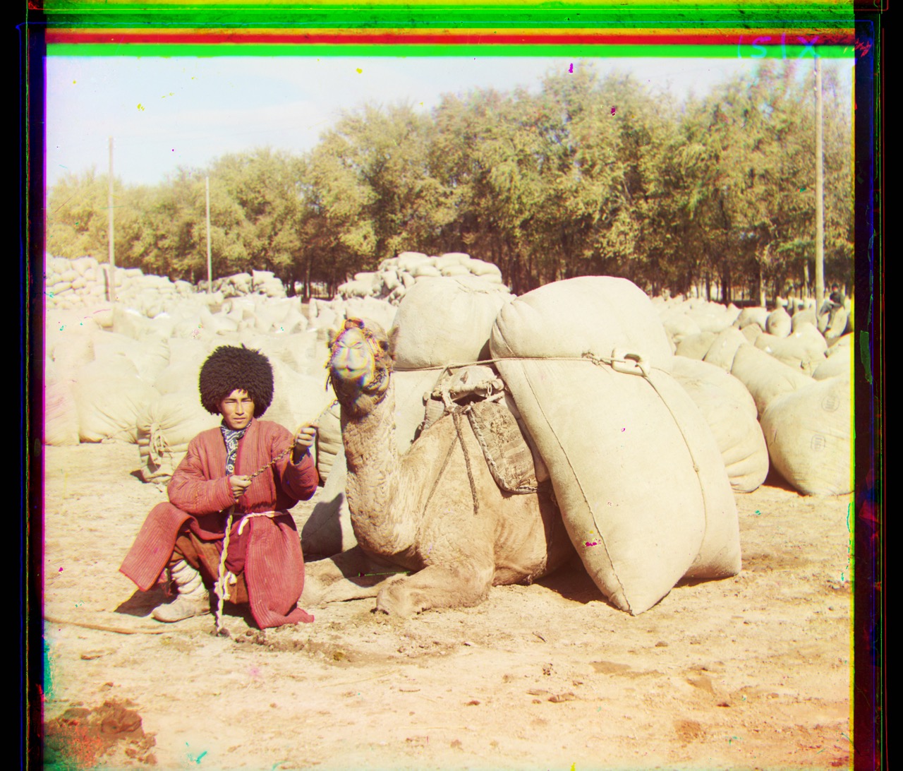
| (##) Image Alignment : Multi-Scale Pyramid Implementation As explained in the single scale solution, multiscale pyramid implementation can reduce the computation to mere few seconds. We can construct an image pyramid to represent the image at multiple scales (scaled by a factor of 2) and the processing is done sequentially starting from the coarsest scale (smallest image) and going down the pyramid until we reach the finest scale. To implement image pyramid, we downscale the original .tiff image to reach the smallest desired image size(256px < smallest image dimension < 512px). We then align the color channels in this image resolution using a (15,15)px window and then use the computed shift as a starting point in the upscaled version. We also reduce the search space from (15,15)px to (13,13)px to (11,11)px as we go towards the finer scale images refining our estimate. For images which are alredy less than 512px , we don't use image pyramids. Initially I computed the similarity and alignment in image(RGB) space, but later I computed the image gradients and used that to compute similarity and alignment. More details on this in the bells and whistles section. I used three different matching scores SSD, NCC and ZNCC. The results of all three have been shared below. An image below shows the construction of a multi-scale pyramid.
Figure: Multi-Scale Pyramid
| SSD loss | NCC Loss| ZNCC Loss | |----------|---------|---|---| ||| |
|
|
| |
| |
| |
|
|
| |
| |
| |
|
|
| |
| |
| |
|
|
| |
| |
| |
|
|
| |
| |
| |
|
|
| |
| |
| |
|
|
| |
| |
| |
|
|
| |
| |
| |
(##) Alignment offsets computed for the images above
| Name | SSD (X offset ,Y offset)| NCC (X offset,Y offset)| ZNCC (X offset,Y offset)|
|-----------------------|------------------------|------------------------|------------------------|
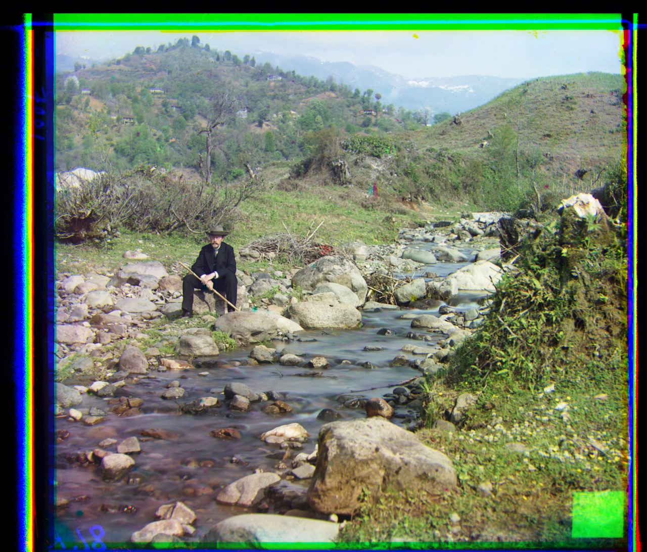
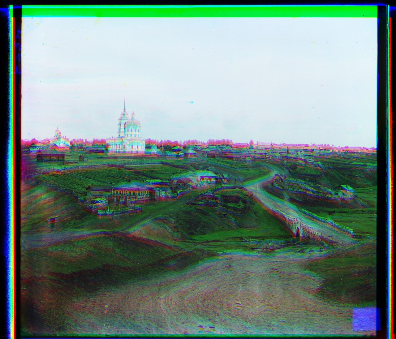
| cathedral.jpg | G: (5,2) R: (12,3) | G: (5,2) R: (12,3) | G: (5,2) R: (12,3) |
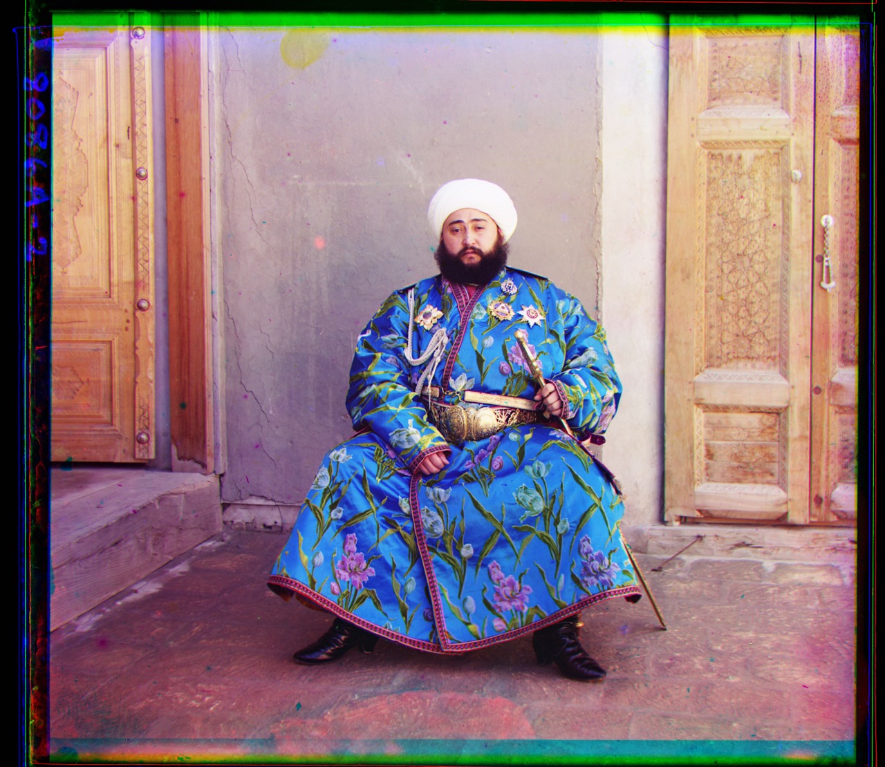
| emir.tif | G: (49,24) R: (105,42) | G: (49,24) R: (105,42) | G: (49,24) R: (105,42) |
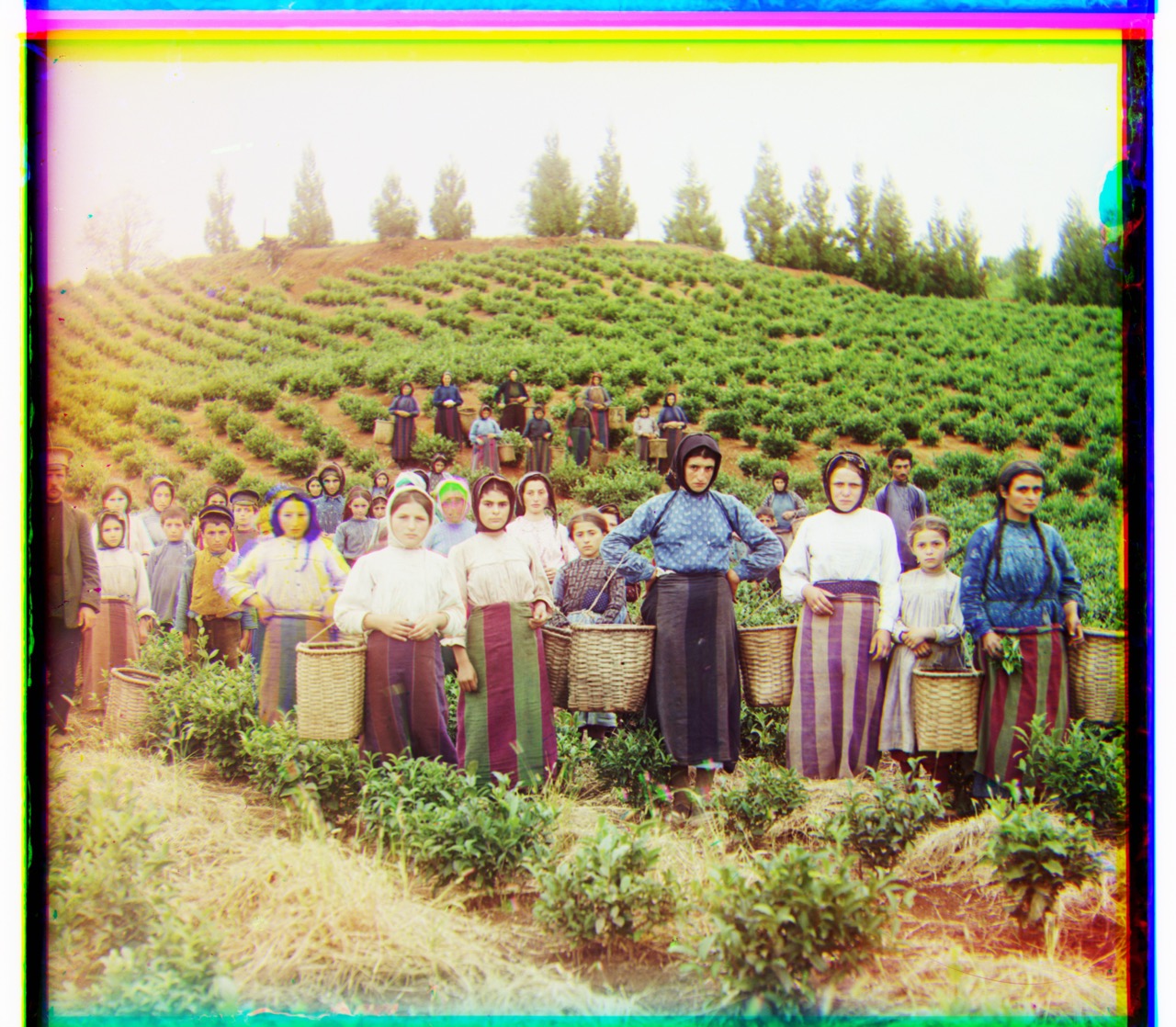
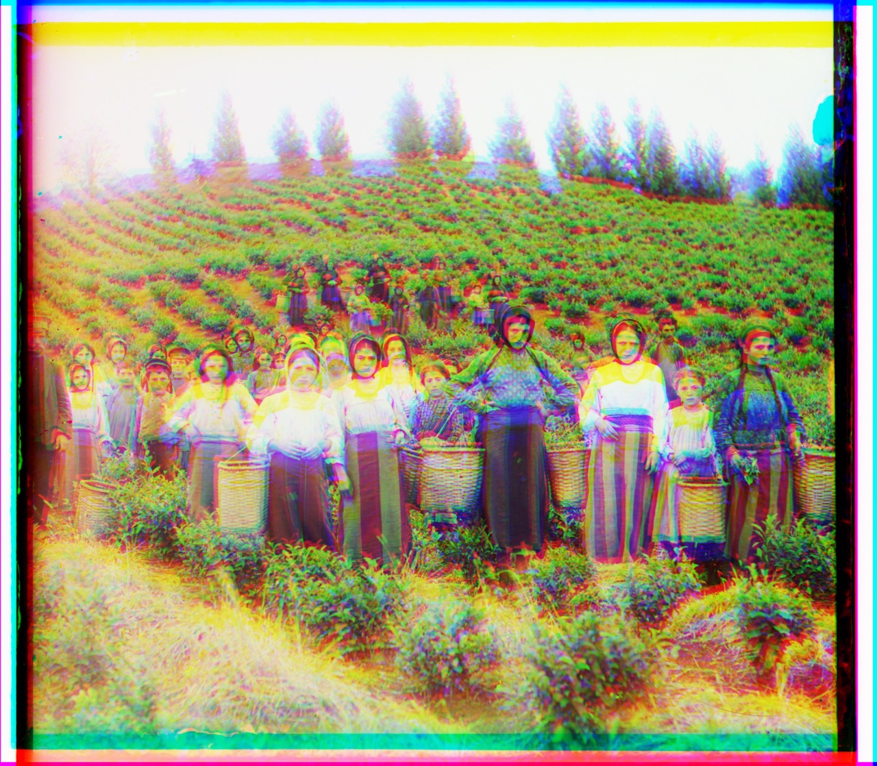
| harvester.tif | G: (60,16) R: (123,12) | G: (60,16) R: (123,12) | G: (60,16) R: (123,12) |
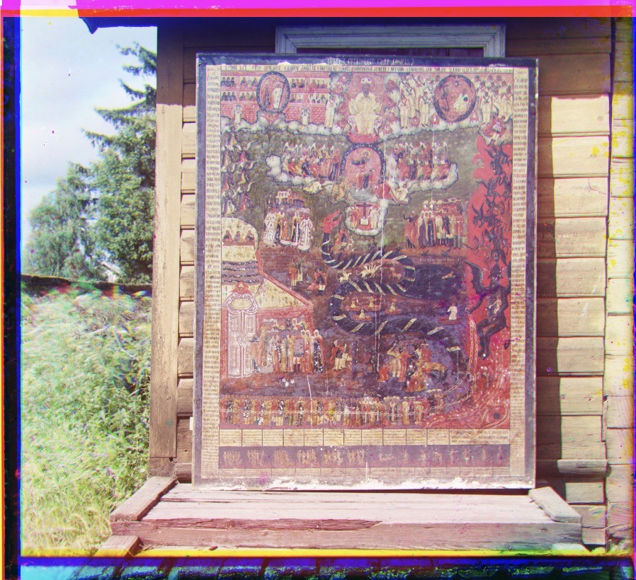
| icon.tif | G: (40,17) R: (89,23) | G: (40,17) R: (89,23) | G: (40,17) R: (89,23) |
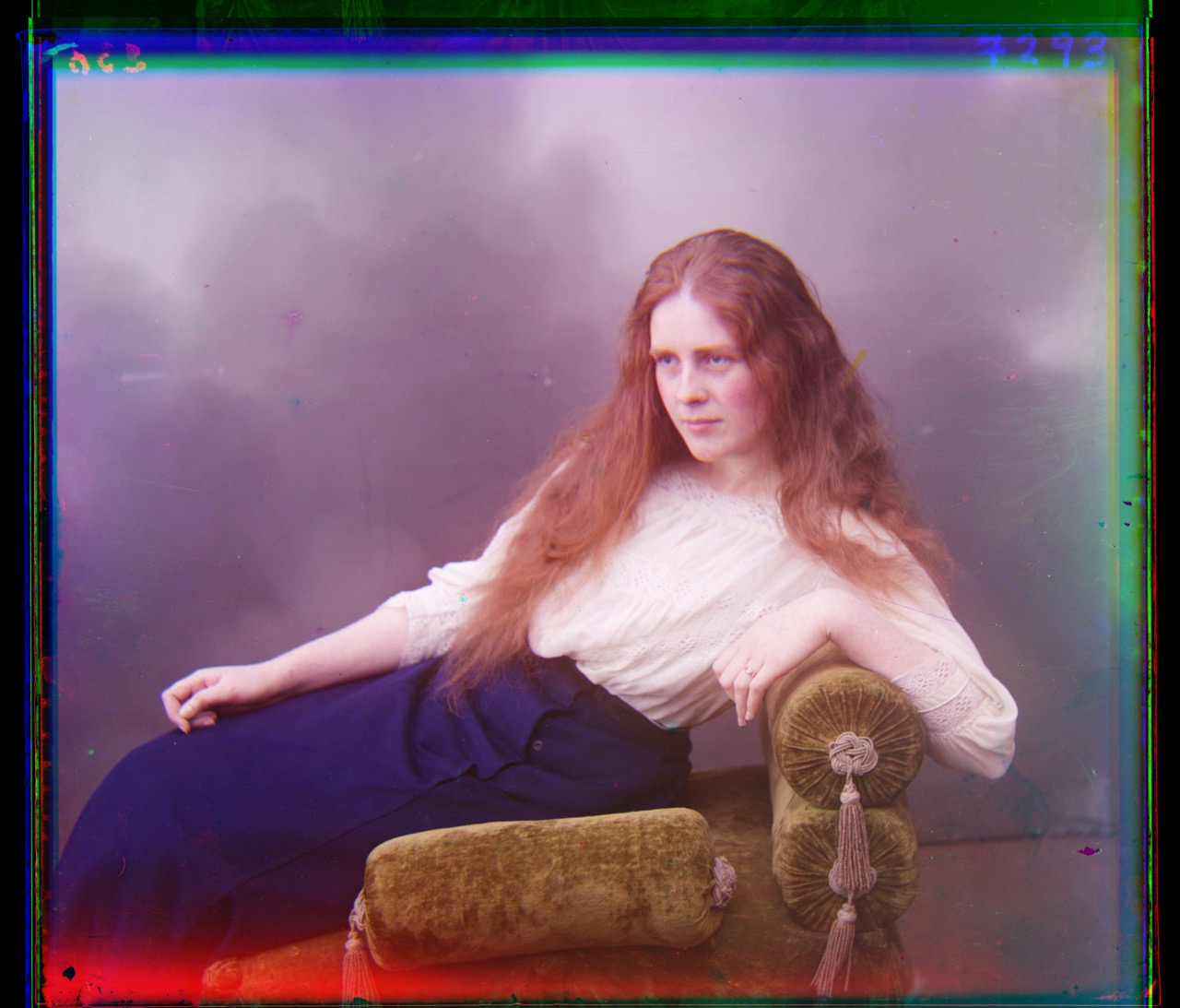
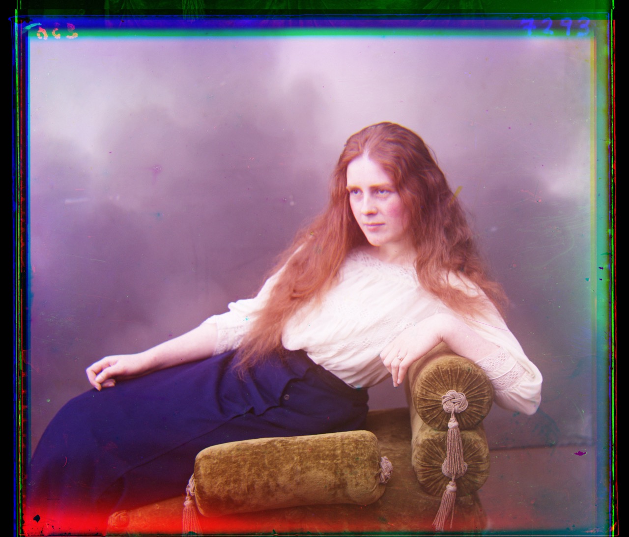
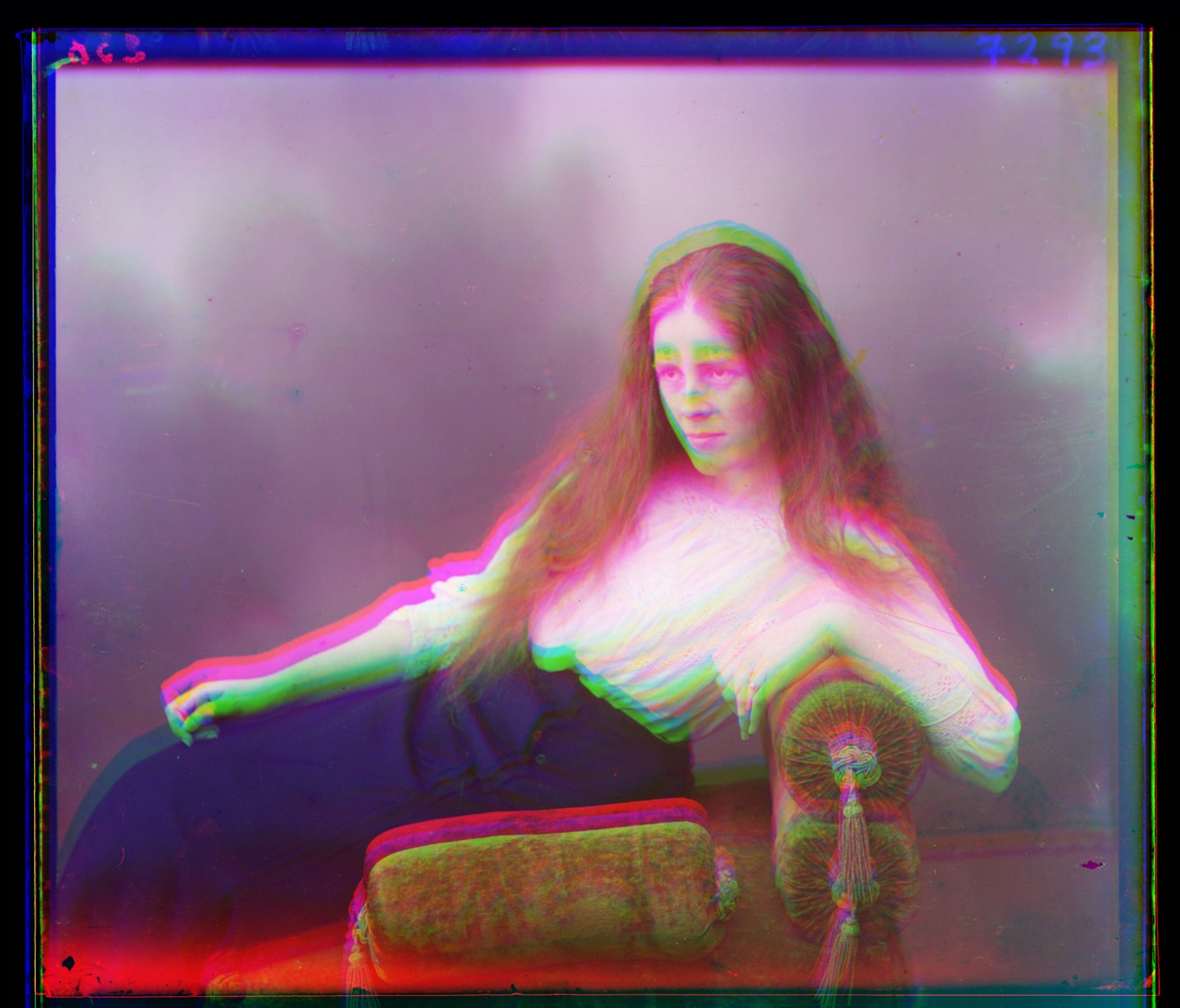
| lady.tif | G: (55,9) R: (118,13) | G: (55,9) R: (118,13) | G: (55,9) R: (118,13) |
| self_portrait.tif | G: (78,29) R: (174,36) | G: (78,29) R: (174,36) | G: (78,29) R: (174,36) |
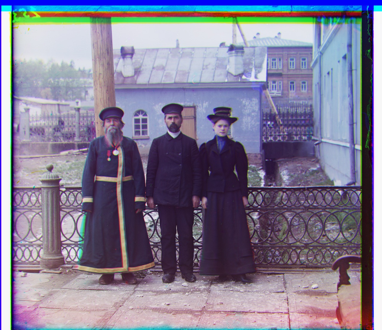
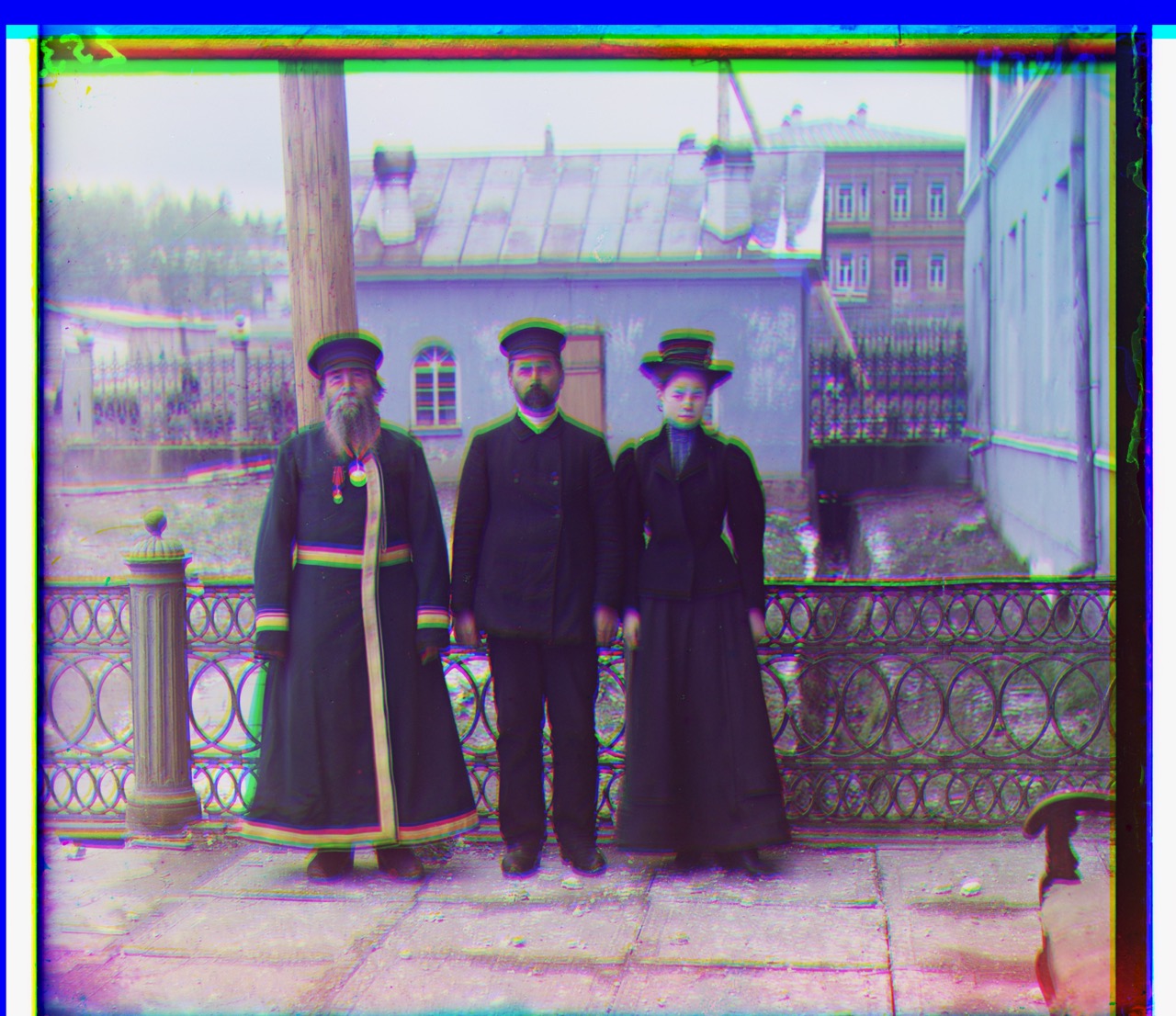
| three_generations.tif | G: (53,13) R: (110,9) | G: (53,13) R: (110,9) | G: (53,13) R: (110,9) |
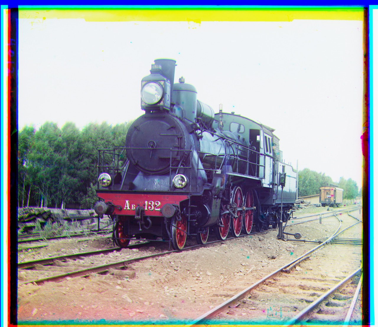
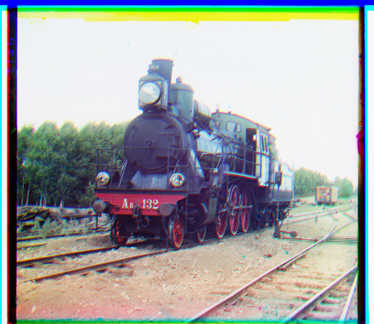
| train.tif | G: (49,6) R: (88,32) | G: (49,6) R: (88,32) | G: (49,6) R: (88,32) |
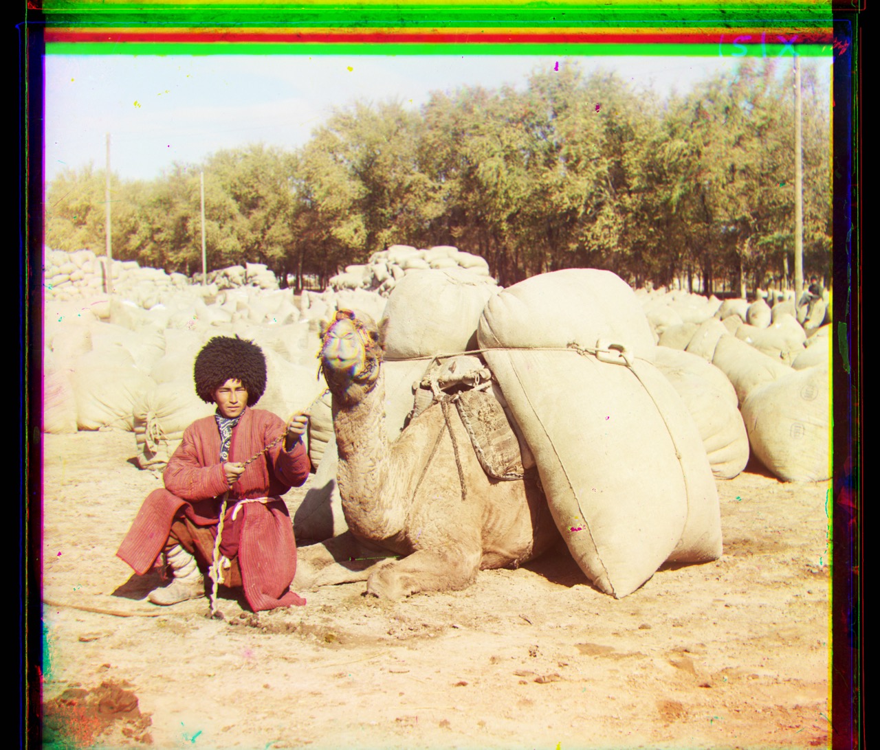
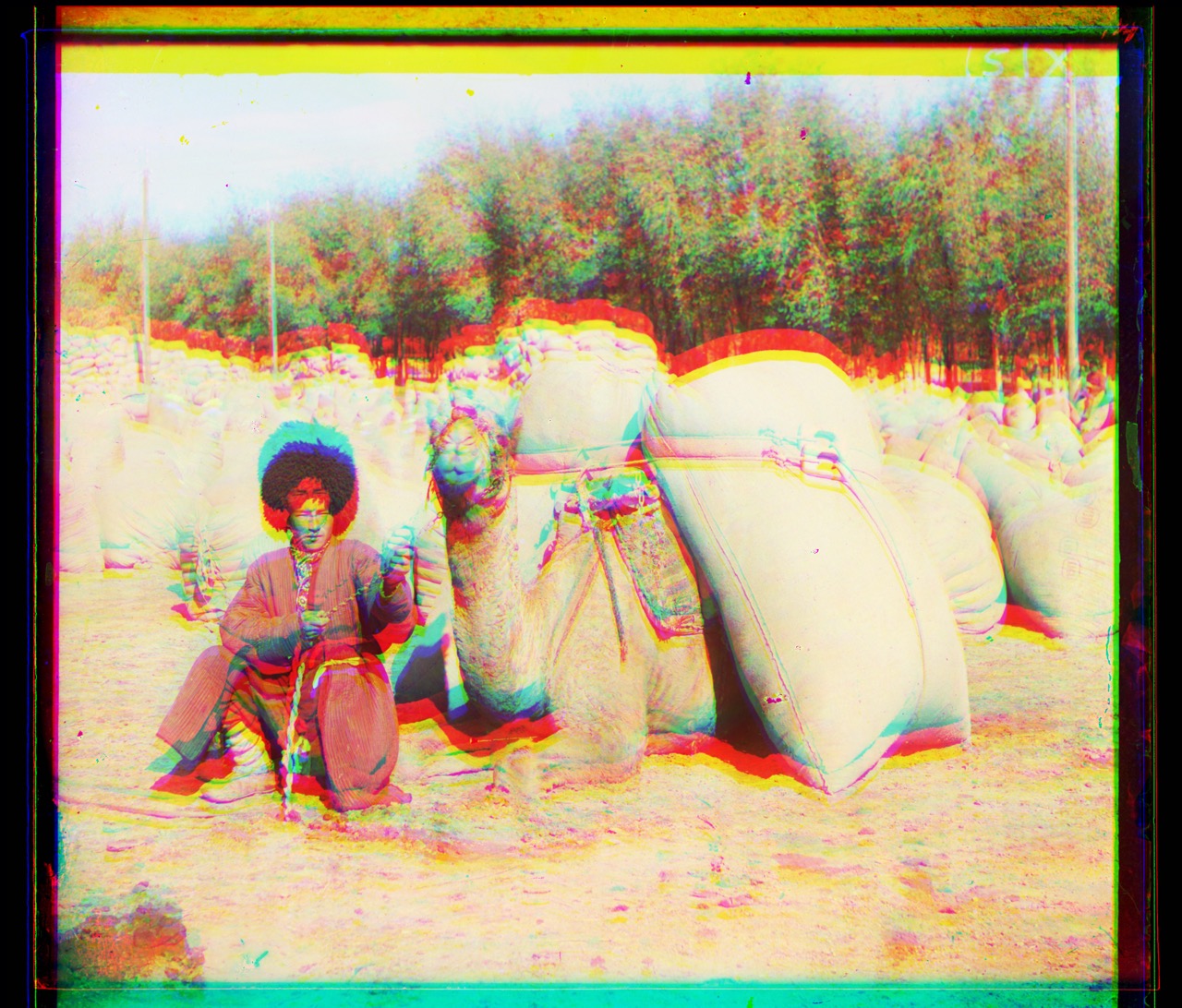
| turkmen.tif | G: (57,22) R: (117,28) | G: (57,22) R: (117,28) | G: (57,22) R: (117,28) |
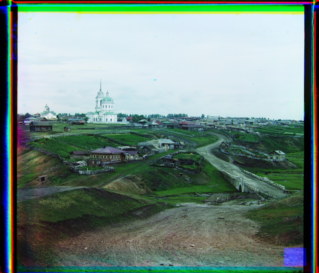
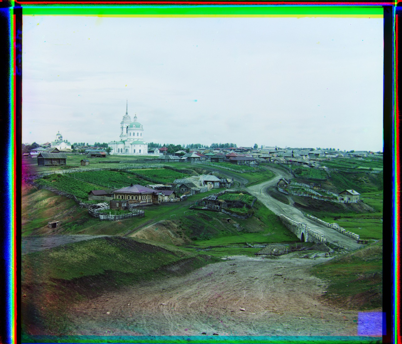
| village.tif | G: (64,10) R: (137,21) | G: (64,10) R: (137,21) | G: (64,10) R: (137,21) |
(#) Extra Credit (Bells and Whistles))
(##) 1. Running code on my own set of images
| SSD loss | NCC Loss| ZNCC Loss |
|----------|---------|---|---|
|
|
(##) Alignment offsets computed for the images above
| Name | SSD (X offset ,Y offset)| NCC (X offset,Y offset)| ZNCC (X offset,Y offset)|
|-----------------------|------------------------|------------------------|------------------------|
| cathedral.jpg | G: (5,2) R: (12,3) | G: (5,2) R: (12,3) | G: (5,2) R: (12,3) |
| emir.tif | G: (49,24) R: (105,42) | G: (49,24) R: (105,42) | G: (49,24) R: (105,42) |
| harvester.tif | G: (60,16) R: (123,12) | G: (60,16) R: (123,12) | G: (60,16) R: (123,12) |
| icon.tif | G: (40,17) R: (89,23) | G: (40,17) R: (89,23) | G: (40,17) R: (89,23) |
| lady.tif | G: (55,9) R: (118,13) | G: (55,9) R: (118,13) | G: (55,9) R: (118,13) |
| self_portrait.tif | G: (78,29) R: (174,36) | G: (78,29) R: (174,36) | G: (78,29) R: (174,36) |
| three_generations.tif | G: (53,13) R: (110,9) | G: (53,13) R: (110,9) | G: (53,13) R: (110,9) |
| train.tif | G: (49,6) R: (88,32) | G: (49,6) R: (88,32) | G: (49,6) R: (88,32) |
| turkmen.tif | G: (57,22) R: (117,28) | G: (57,22) R: (117,28) | G: (57,22) R: (117,28) |
| village.tif | G: (64,10) R: (137,21) | G: (64,10) R: (137,21) | G: (64,10) R: (137,21) |
(#) Extra Credit (Bells and Whistles))
(##) 1. Running code on my own set of images
| SSD loss | NCC Loss| ZNCC Loss |
|----------|---------|---|---|
| |||
|
|||
| |||
|
|||
| |||
|
|||
| |||
| Name | SSD (X offset ,Y offset)| NCC (X offset,Y offset)| ZNCC (X offset,Y offset)|
|-----------------------|------------------------|------------------------|------------------------|
| artpiece.jpg | G: (13,50) R: (19,113) | G: (13,50) R: (19,113) | G: (13,50) R: (19,113) |
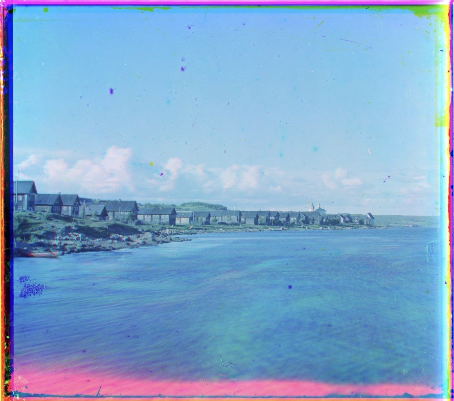
| beachtown.tif | G: (15,16) R: (28,33) | G: (15,16) R: (28,33) | G: (15,16) R: (28,33) |
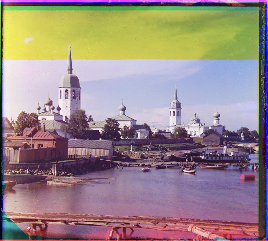
| city.tif | G: (21,13) R: (27,36) | G: (21,13) R: (27,36) | G: (21,13) R: (27,36) |
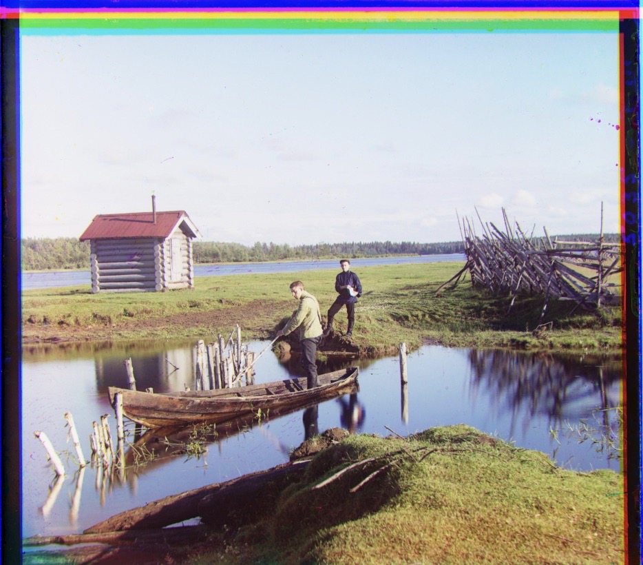
| pond.tif | G: (-7,13) R: (-13,135) | G: (-7,13) R: (-13,135) | G: (-7,13) R: (-13,135) |
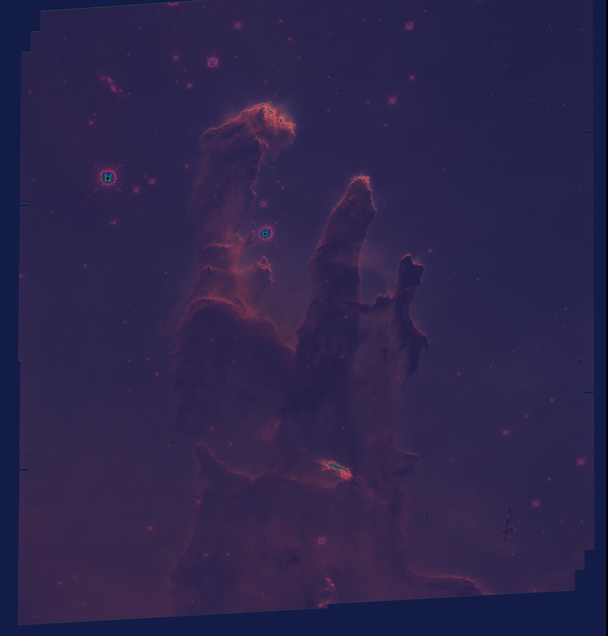
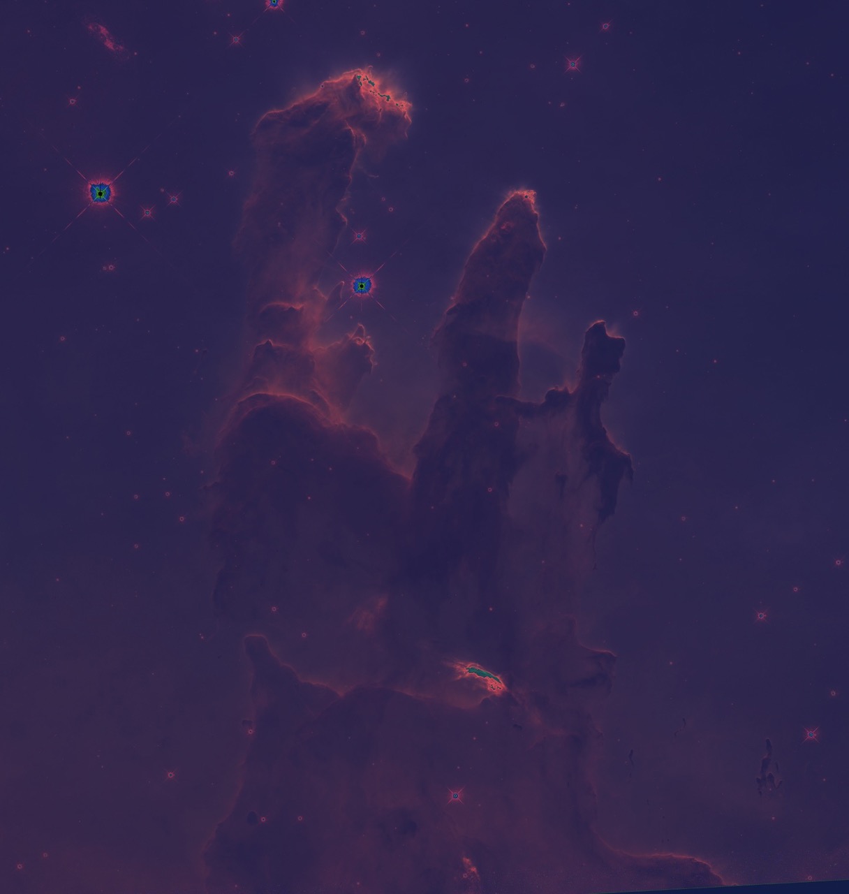
(##) 2. Running on astro images taken from Hubble telescope
This image have been taken by Hubble telescope and is known as three pillars. I stacked them togther using my algorithm
| Before Crop | After Crop |
|-----------------------|------------------------|
|
|||
| Name | SSD (X offset ,Y offset)| NCC (X offset,Y offset)| ZNCC (X offset,Y offset)|
|-----------------------|------------------------|------------------------|------------------------|
| artpiece.jpg | G: (13,50) R: (19,113) | G: (13,50) R: (19,113) | G: (13,50) R: (19,113) |
| beachtown.tif | G: (15,16) R: (28,33) | G: (15,16) R: (28,33) | G: (15,16) R: (28,33) |
| city.tif | G: (21,13) R: (27,36) | G: (21,13) R: (27,36) | G: (21,13) R: (27,36) |
| pond.tif | G: (-7,13) R: (-13,135) | G: (-7,13) R: (-13,135) | G: (-7,13) R: (-13,135) |
(##) 2. Running on astro images taken from Hubble telescope
This image have been taken by Hubble telescope and is known as three pillars. I stacked them togther using my algorithm
| Before Crop | After Crop |
|-----------------------|------------------------|
| |
| |
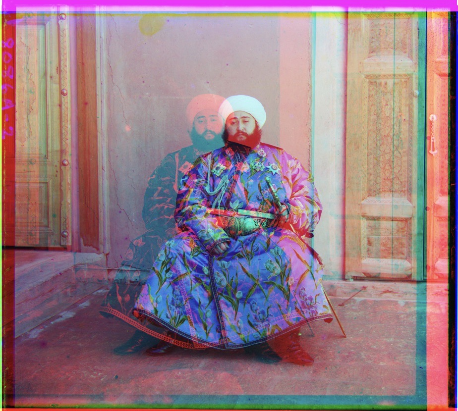
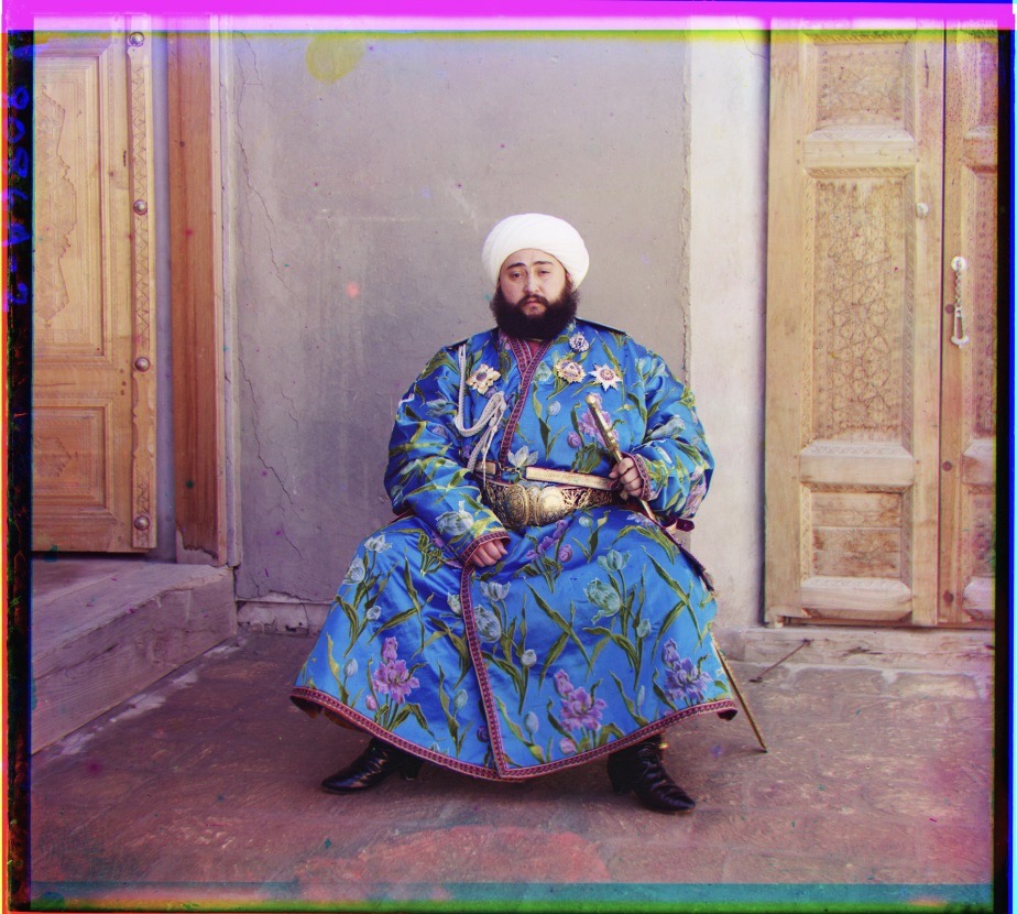
(##) 3. Computing similarity in color space vs computing similarity in gradient space
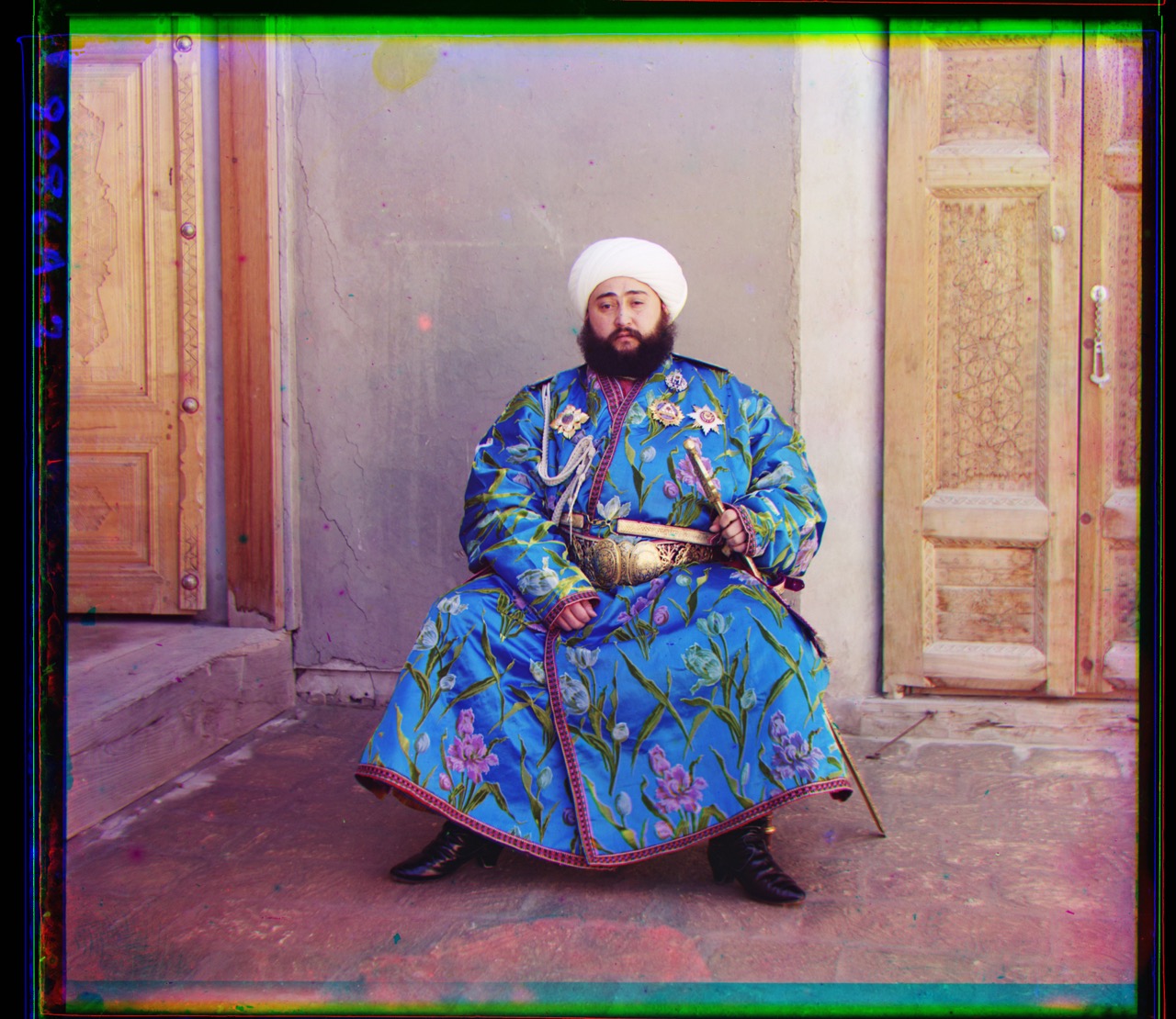
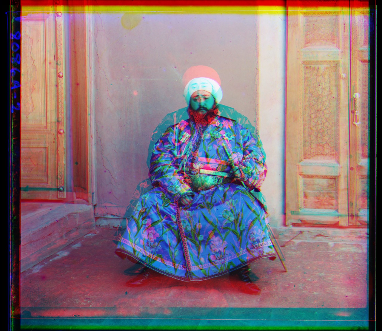
This section shows that the alignments become particularly better when the alignment is in gradient space as opposed to in color space. emir.tiff caused
issues when it came to aligning the red channel with blue channel. Neither NCC, ZNCC worked in this case.
So, I computed the image gradients and then aligned them. Image on the right shows proper alignment of the towards.
| Similarity in color space| Similarity in gradient space|
|-----------------------|------------------------|
|
|
(##) 3. Computing similarity in color space vs computing similarity in gradient space
This section shows that the alignments become particularly better when the alignment is in gradient space as opposed to in color space. emir.tiff caused
issues when it came to aligning the red channel with blue channel. Neither NCC, ZNCC worked in this case.
So, I computed the image gradients and then aligned them. Image on the right shows proper alignment of the towards.
| Similarity in color space| Similarity in gradient space|
|-----------------------|------------------------|
| |
| |
(##) 4. Pytorch Implementation
Pytorch and Numpy have similar functions in their API. The pytorch implementation, remains the same as the numpy implementation. For cropping the image, I used centercrop from
torchvision transforms instead of using indexing like in numpy based implementation.
Similarity measures like NCC, ZNCC and SSD were also computed as torch tensors instead of numpy nd arrays.
The output of the implementation is same as the one in numpy. There is no observed change in alignment.
| SSD loss | NCC Loss| ZNCC Loss |
|----------|---------|---|---|
||||
||||
||||
||||
||||
||||
||||
||||
||||
(##) Alignment offsets computed for the images above
| Name | SSD (X offset ,Y offset)| NCC (X offset,Y offset)| ZNCC (X offset,Y offset)|
|-----------------------|------------------------|------------------------|------------------------|
| cathedral.jpg | G: (5,2) R: (12,3) | G: (5,2) R: (12,3) | G: (5,2) R: (12,3) |
| emir.tif | G: (49,24) R: (105,42) | G: (49,24) R: (105,42) | G: (49,24) R: (105,42) |
| harvester.tif | G: (60,16) R: (123,12) | G: (60,16) R: (123,12) | G: (60,16) R: (123,12) |
| icon.tif | G: (40,17) R: (89,23) | G: (40,17) R: (89,23) | G: (40,17) R: (89,23) |
| lady.tif | G: (55,9) R: (118,13) | G: (55,9) R: (118,13) | G: (55,9) R: (118,13) |
| self_portrait.tif | G: (78,29) R: (174,36) | G: (78,29) R: (174,36) | G: (78,29) R: (174,36) |
| three_generations.tif | G: (53,13) R: (110,9) | G: (53,13) R: (110,9) | G: (53,13) R: (110,9) |
| train.tif | G: (49,6) R: (88,32) | G: (49,6) R: (88,32) | G: (49,6) R: (88,32) |
| turkmen.tif | G: (57,22) R: (117,28) | G: (57,22) R: (117,28) | G: (57,22) R: (117,28) |
| village.tif | G: (64,10) R: (137,21) | G: (64,10) R: (137,21) | G: (64,10) R: (137,21) |
(#) Bells and Whistles using own ideas
(##) Image similarty using discrete fourier transforms (Chi squared Shift)
Here, I have used Discrete fourier Transform to regsiter or align the images. DFT registers two images (2-D rigid translation) within a fraction of a pixel specified by the user.
Instead of computing a zero-padded FFT (fast Fourier transform), this code uses selective upsampling by a matrix-multiply DFT (discrete FT) to dramatically reduce computation time and memory without sacrificing accuracy.
With this procedure all the image points are used to compute the upsampled cross-correlation in a very small neighborhood around its peak. This algorithm is referred to as the single-step DFT algorithm in [1].
Original Papaer: [1] Manuel Guizar-Sicairos, Samuel T. Thurman, and James R. Fienup, "Efficient subpixel image registration algorithms," Opt. Lett. 33, 156-158 (2008).
Important thing to note is that even for 4K images, I dont use image pyramids and despite that the compute time is almost 1/3rd of that of my original implementation.
The times have been shared in the next section.
For implementation of this I have used the library image registration.
More details can be found here
| Results from DFT (chi squared shift)|Results from DFT (chi squared shift)|
|-----------------------|------------------------------|
|
|
(##) 4. Pytorch Implementation
Pytorch and Numpy have similar functions in their API. The pytorch implementation, remains the same as the numpy implementation. For cropping the image, I used centercrop from
torchvision transforms instead of using indexing like in numpy based implementation.
Similarity measures like NCC, ZNCC and SSD were also computed as torch tensors instead of numpy nd arrays.
The output of the implementation is same as the one in numpy. There is no observed change in alignment.
| SSD loss | NCC Loss| ZNCC Loss |
|----------|---------|---|---|
||||
||||
||||
||||
||||
||||
||||
||||
||||
(##) Alignment offsets computed for the images above
| Name | SSD (X offset ,Y offset)| NCC (X offset,Y offset)| ZNCC (X offset,Y offset)|
|-----------------------|------------------------|------------------------|------------------------|
| cathedral.jpg | G: (5,2) R: (12,3) | G: (5,2) R: (12,3) | G: (5,2) R: (12,3) |
| emir.tif | G: (49,24) R: (105,42) | G: (49,24) R: (105,42) | G: (49,24) R: (105,42) |
| harvester.tif | G: (60,16) R: (123,12) | G: (60,16) R: (123,12) | G: (60,16) R: (123,12) |
| icon.tif | G: (40,17) R: (89,23) | G: (40,17) R: (89,23) | G: (40,17) R: (89,23) |
| lady.tif | G: (55,9) R: (118,13) | G: (55,9) R: (118,13) | G: (55,9) R: (118,13) |
| self_portrait.tif | G: (78,29) R: (174,36) | G: (78,29) R: (174,36) | G: (78,29) R: (174,36) |
| three_generations.tif | G: (53,13) R: (110,9) | G: (53,13) R: (110,9) | G: (53,13) R: (110,9) |
| train.tif | G: (49,6) R: (88,32) | G: (49,6) R: (88,32) | G: (49,6) R: (88,32) |
| turkmen.tif | G: (57,22) R: (117,28) | G: (57,22) R: (117,28) | G: (57,22) R: (117,28) |
| village.tif | G: (64,10) R: (137,21) | G: (64,10) R: (137,21) | G: (64,10) R: (137,21) |
(#) Bells and Whistles using own ideas
(##) Image similarty using discrete fourier transforms (Chi squared Shift)
Here, I have used Discrete fourier Transform to regsiter or align the images. DFT registers two images (2-D rigid translation) within a fraction of a pixel specified by the user.
Instead of computing a zero-padded FFT (fast Fourier transform), this code uses selective upsampling by a matrix-multiply DFT (discrete FT) to dramatically reduce computation time and memory without sacrificing accuracy.
With this procedure all the image points are used to compute the upsampled cross-correlation in a very small neighborhood around its peak. This algorithm is referred to as the single-step DFT algorithm in [1].
Original Papaer: [1] Manuel Guizar-Sicairos, Samuel T. Thurman, and James R. Fienup, "Efficient subpixel image registration algorithms," Opt. Lett. 33, 156-158 (2008).
Important thing to note is that even for 4K images, I dont use image pyramids and despite that the compute time is almost 1/3rd of that of my original implementation.
The times have been shared in the next section.
For implementation of this I have used the library image registration.
More details can be found here
| Results from DFT (chi squared shift)|Results from DFT (chi squared shift)|
|-----------------------|------------------------------|
| |
| |
|
|
| |
|
|
| |
| |
|
|
| |
| |
|
|
| |
(###) Alignment Offsets
| Name | Chi Squared Shift Offsets|
|-----------------------|------------------------|
|emir.tif | G (48.572265625, 23.552734375) R (105.361328125, 41.634765625)|
|three_generations.tif | G (52.814453125, 12.595703125) R (109.568359375, 8.658203125)|
|train.tif | G (48.771484375, 6.259765625) R (88.123046875, 32.244140625)|
|icon.tif | G (39.466796875, 16.541015625) R (88.634765625, 22.705078125)|
|cathedral.jpg | G (4.958984375, 2.232421875) R (11.732421875, 3.052734375)|
|village.tif | G (64.369140625, 10.376953125) R (137.302734375, 21.451171875)|
|self_portrait.tif | G (77.576171875, 28.634765625) R (174.494140625, 36.447265625)|
|harvesters.tif | G (59.720703125, 15.970703125) R (122.755859375, 12.435546875)|
|lady.tif | G (55.259765625, 8.814453125) R (118.498046875, 12.681640625)|
|turkmen.tif | G (56.857421875, 21.892578125) R (117.255859375, 28.490234375)|
(###) Processing Times
The table below shows a comparison between chi square shift and normal shift implemented in this Assignment
It can be clearly seen that the chi squared shift is much faster than NCC implementation
| Name | Chi Squared Shift time (s)| NCC time(s) |
|-----------------------|------------------------|---|
|emir.tif | 3.27 | 9.83 |
|three_generations.tif | 2.89 | 8.83|
|train.tif | 3.12| 9.77 |
|icon.tif |2.24 | 6.99 |
|cathedral.jpg | 2.07 | 6.68|
|village.tif | 3.44 | 10.7 |
|self_portrait.tif | 2.63 | 7.96 |
|harvesters.tif | 2.08 | 7.34 |
|lady.tif | 1.76 | 6.82 |
|turkmen.tif | 2.55 | 7.43 |
(##) Image Registration using optical flow
In this method, I tried using optical flow using iterative Lucas Kanade algorithm. By definition, the optical flow is the vector field (u, v) verifying image1(x+u, y+v) = image0(x, y), where (image0, image1) is a couple of consecutive 2D frames from a sequence.
In our case these consecutive frames can be thought of two channels in our image. This vector field can then be used for registration by image warping.
To display registration results, an RGB image is constructed by assigning the result of the registration to the red channel and the target image to the green and blue channels. A perfect registration results in a gray level image while misregistred pixels appear colored in the constructed RGB image.
I used the scipy.ndimage package for this implementation. However the results of the optical flow are comparable to that of DFT and normal SSD, NCC based algorithms.
I tried computing optical flow in both spaces- color and gradient. It worked well in color space and not so well in gradient space. The computation time is also higher compared to any of the methods
mentioned in this project. Images below show optical flow registration using color and gradient based similarity.
| Optical flow alignment(color space) |Optical flow alignment(gradient space) |
|-----------------------|------------------------------|
||
|
(###) Alignment Offsets
| Name | Chi Squared Shift Offsets|
|-----------------------|------------------------|
|emir.tif | G (48.572265625, 23.552734375) R (105.361328125, 41.634765625)|
|three_generations.tif | G (52.814453125, 12.595703125) R (109.568359375, 8.658203125)|
|train.tif | G (48.771484375, 6.259765625) R (88.123046875, 32.244140625)|
|icon.tif | G (39.466796875, 16.541015625) R (88.634765625, 22.705078125)|
|cathedral.jpg | G (4.958984375, 2.232421875) R (11.732421875, 3.052734375)|
|village.tif | G (64.369140625, 10.376953125) R (137.302734375, 21.451171875)|
|self_portrait.tif | G (77.576171875, 28.634765625) R (174.494140625, 36.447265625)|
|harvesters.tif | G (59.720703125, 15.970703125) R (122.755859375, 12.435546875)|
|lady.tif | G (55.259765625, 8.814453125) R (118.498046875, 12.681640625)|
|turkmen.tif | G (56.857421875, 21.892578125) R (117.255859375, 28.490234375)|
(###) Processing Times
The table below shows a comparison between chi square shift and normal shift implemented in this Assignment
It can be clearly seen that the chi squared shift is much faster than NCC implementation
| Name | Chi Squared Shift time (s)| NCC time(s) |
|-----------------------|------------------------|---|
|emir.tif | 3.27 | 9.83 |
|three_generations.tif | 2.89 | 8.83|
|train.tif | 3.12| 9.77 |
|icon.tif |2.24 | 6.99 |
|cathedral.jpg | 2.07 | 6.68|
|village.tif | 3.44 | 10.7 |
|self_portrait.tif | 2.63 | 7.96 |
|harvesters.tif | 2.08 | 7.34 |
|lady.tif | 1.76 | 6.82 |
|turkmen.tif | 2.55 | 7.43 |
(##) Image Registration using optical flow
In this method, I tried using optical flow using iterative Lucas Kanade algorithm. By definition, the optical flow is the vector field (u, v) verifying image1(x+u, y+v) = image0(x, y), where (image0, image1) is a couple of consecutive 2D frames from a sequence.
In our case these consecutive frames can be thought of two channels in our image. This vector field can then be used for registration by image warping.
To display registration results, an RGB image is constructed by assigning the result of the registration to the red channel and the target image to the green and blue channels. A perfect registration results in a gray level image while misregistred pixels appear colored in the constructed RGB image.
I used the scipy.ndimage package for this implementation. However the results of the optical flow are comparable to that of DFT and normal SSD, NCC based algorithms.
I tried computing optical flow in both spaces- color and gradient. It worked well in color space and not so well in gradient space. The computation time is also higher compared to any of the methods
mentioned in this project. Images below show optical flow registration using color and gradient based similarity.
| Optical flow alignment(color space) |Optical flow alignment(gradient space) |
|-----------------------|------------------------------|
|| |
||
|
|| |
||
|
|| |
||
|
|| |
||
|
|| |
||
|
|| |
||
|
|| |
||
|
|| |
|