Introduction
Image restoration has seen a great deal of progress, with the creation of contemporary photographs using filters like denoising, colorization, and super resolution on old, grainy, black-and-white photos. In addition to this, the creators of Time-Travel Rephotography employ StyleGAN2 to transpose outdated images into a contemporary high-resolution image space. In order to imitate the characteristics of vintage cameras and the aging process of film, they use a physically based film deterioration operator. They eventually create the model output image using contextual loss and color transfer loss. The process of converting ancient photos to a modern versions gives the audience a perspective of how someone would have looked during the time and helps revisualize the aspect of color as well.Problem Description
The main objective of the Time-Travel Rephotography paper is to replicate the experience of traveling back in time and capturing portraits of historical figures
with modern cameras. The focus is on portraits captured around a century ago, in the early days of photography, which are difficult to restore due to the loss of
quality caused by aging and the limitations of early photographic technology.
To replicate the experience of rephotographing historical figures with modern cameras, it is important to consider the differences in color sensitivity between
antique and modern films, as well as factors such as blur, fading, poor exposure, low resolution, and other artifacts associated with antique photos. The Time-Travel
Rephotography paper does a great job at generating modern photographs by considering artifact removal, colorization, super-resolution, and contrast adjustment in one
unified framework. This framework works much better than other state-of-the-art image restoration filters. They also display rephotographed portraits of many historical
figures including presidents, authors, artists, and scientists. This is achieved by using StyleGAN2. Their approach involves creating a counterpart of an input antique
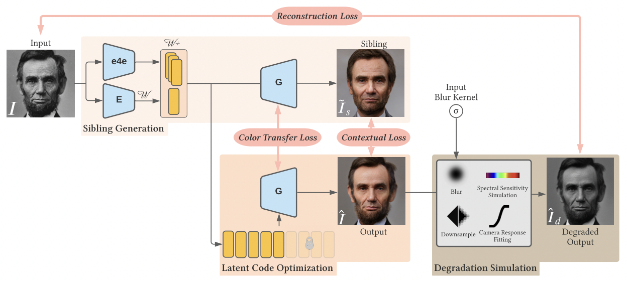
photograph in the StyleGAN2 latent space. To achieve this, style mixing is used, where the predictions from two feed-forward encoders: one that models face identity (e4e)
and another that models face color (E) is combined. This generates a sibling image that is optimized to match the input photograph after undergoing degradation to
simulate an antique image. The color, contrast, and skin textures of the sibling image is used to guide the optimization of the latent code. The whole system diagram
can be seen in the below figure (directly taken from the paper) -
Inspired by this paper, we first perform an error analysis on the cases where this model fails to perform well. After this, we implement a few techniques which improves
the performance of the model (including the quality of the modern images produced). The results from our error analysis as well as proposed improvements are listed in
the next sections.
Scope for Improvements
Based on our review of the work Time Travel Rephotography we decided to experiment
with a few potential improvements that we can try out in order to improve the quality of the images. The scopes
for improvement are as listed below:
- Reduce effect of brightness and contrast of the input image on the predicted skin color : We experiment with using Huber Loss instead of Smooth L1 Loss.
- Improve inaccurately predicting skin texture from images in certain cases : We experiment with a preprocessing strategy and different loss combinations. We also try out noise regularization and changing its hyperparameters.
- Utilizing L2 Loss for reconstruction instead of L1 Loss : In order to better capture the finer details, we implement the L2 Loss instead of the L1 Loss for the reconstruction and determine whether there is an improvement.
- Using a preprocessing pipeline to remove artifacts: We noticed that accessories present around people's faces such as hats and extensive beards tend to be not reconstructed correctly. Hence we try out a preprocessing strategy based on an attention based GAN in order to capture these details better.
- Improve the strength of noise regularizer: We came up with different ways of reducing the noise regularizer strength that optimizes the w+ global style codes in an aim to focus more on local features.
- Using a better interpolation method: We experimented with a bicubic interpolation method instead of bilinear to see if it provides more finer details.
Examples of Bad Results
We performed some error analysis by inspecting how the results change by giving varied antique images. We chose examples which had artifacts such as hats or glasses.
A few examples did not have enough contrast in the image or where the brightness was less. Below are a few failure cases we identified -
-
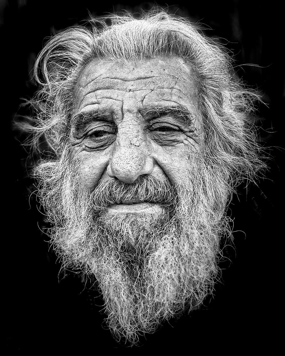
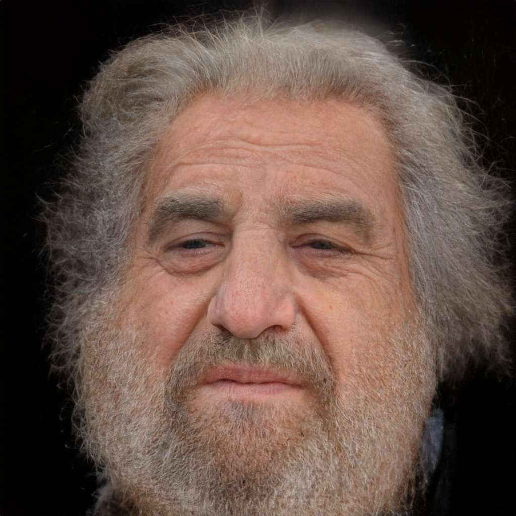
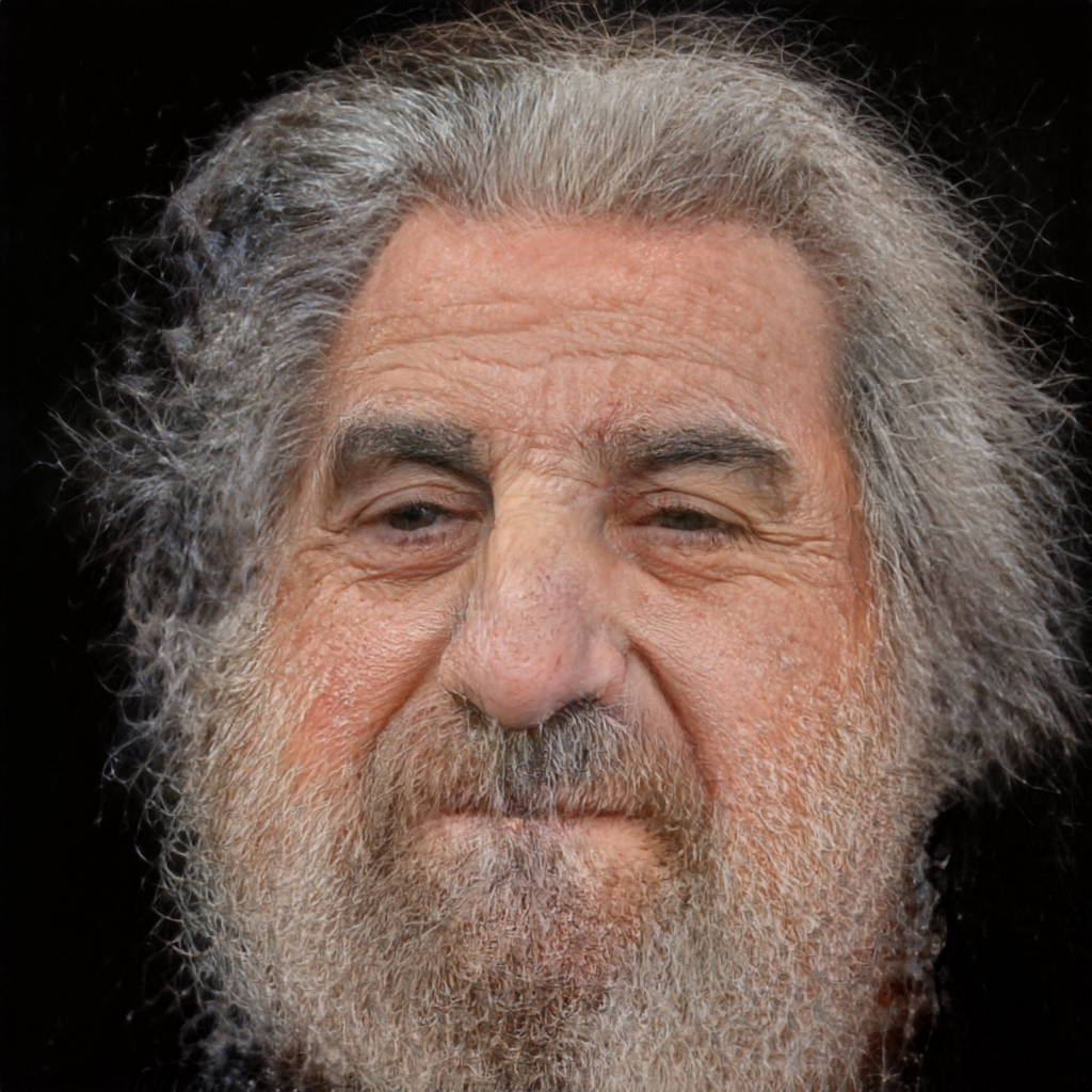
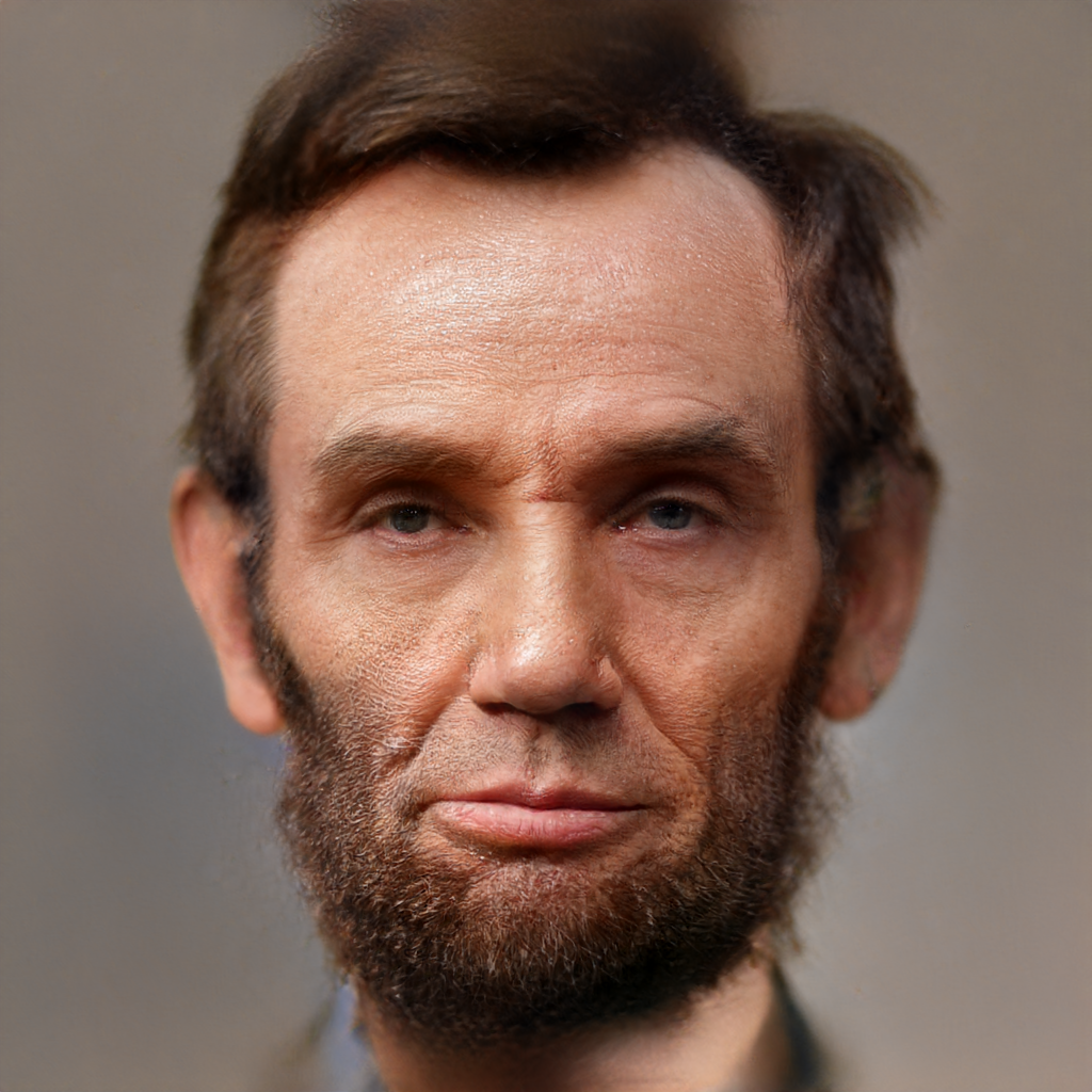
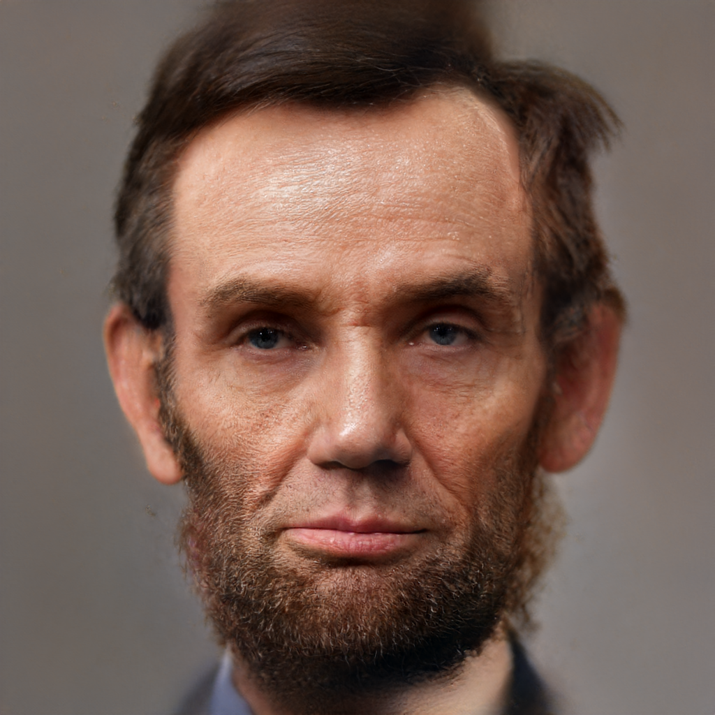
In this example, the contrast of the man's beard with the background is very less. Hence, in the modern version of the photo, the part of the beard which clashes with
the background has been erased. A similar thing has happened with the man's hair as well.
Original Old Image
Reconstructed Image
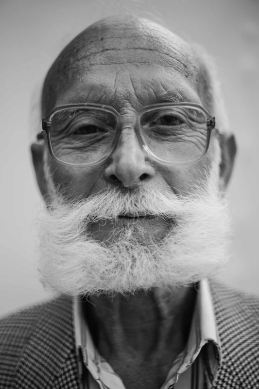
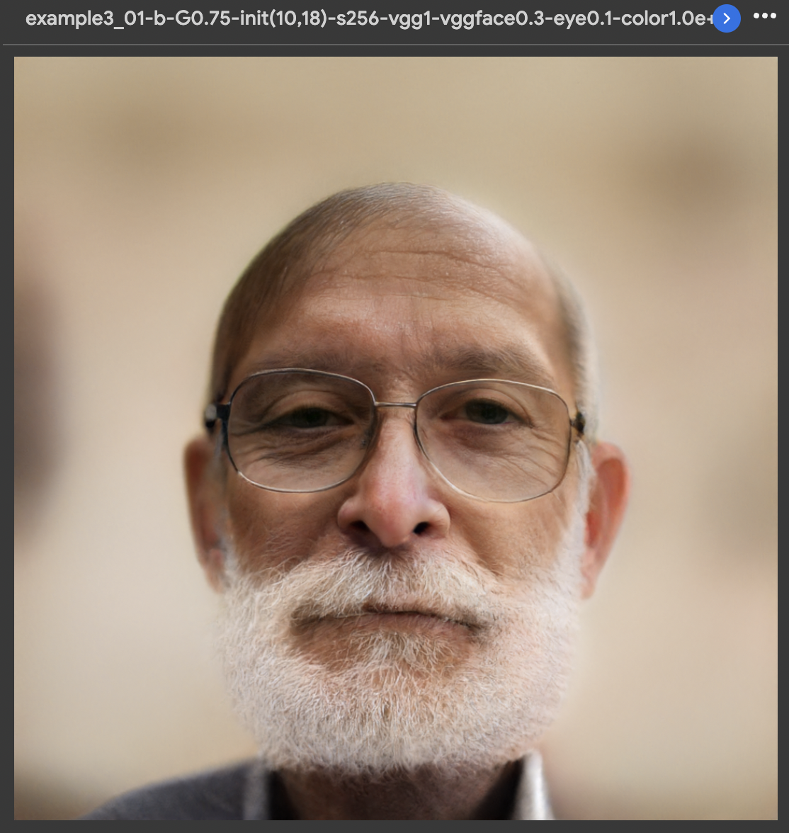
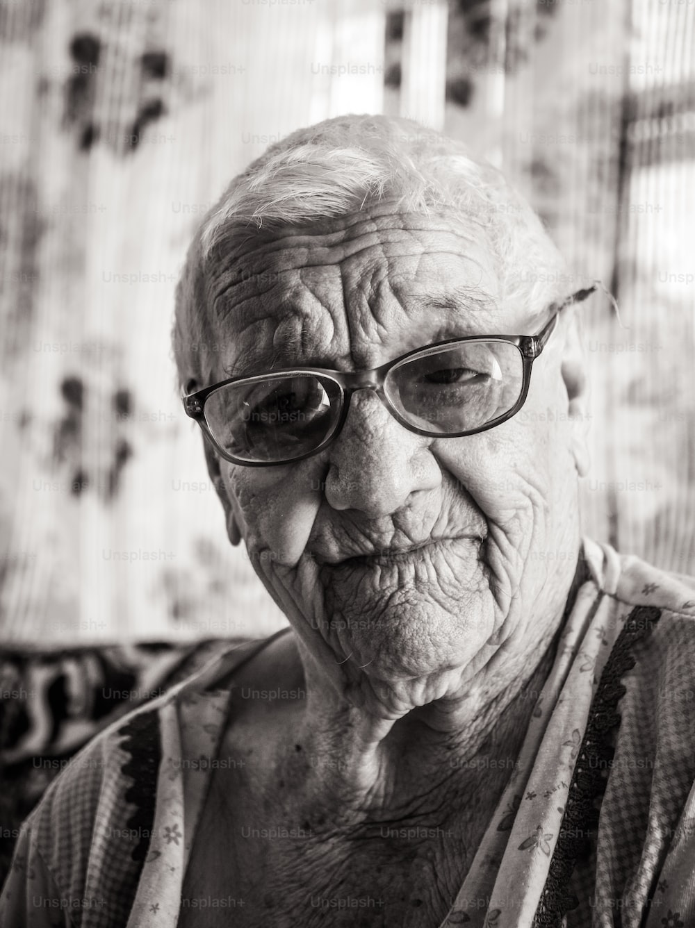
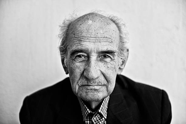
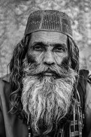
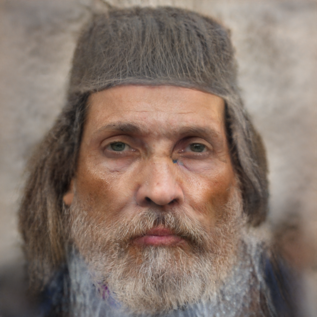
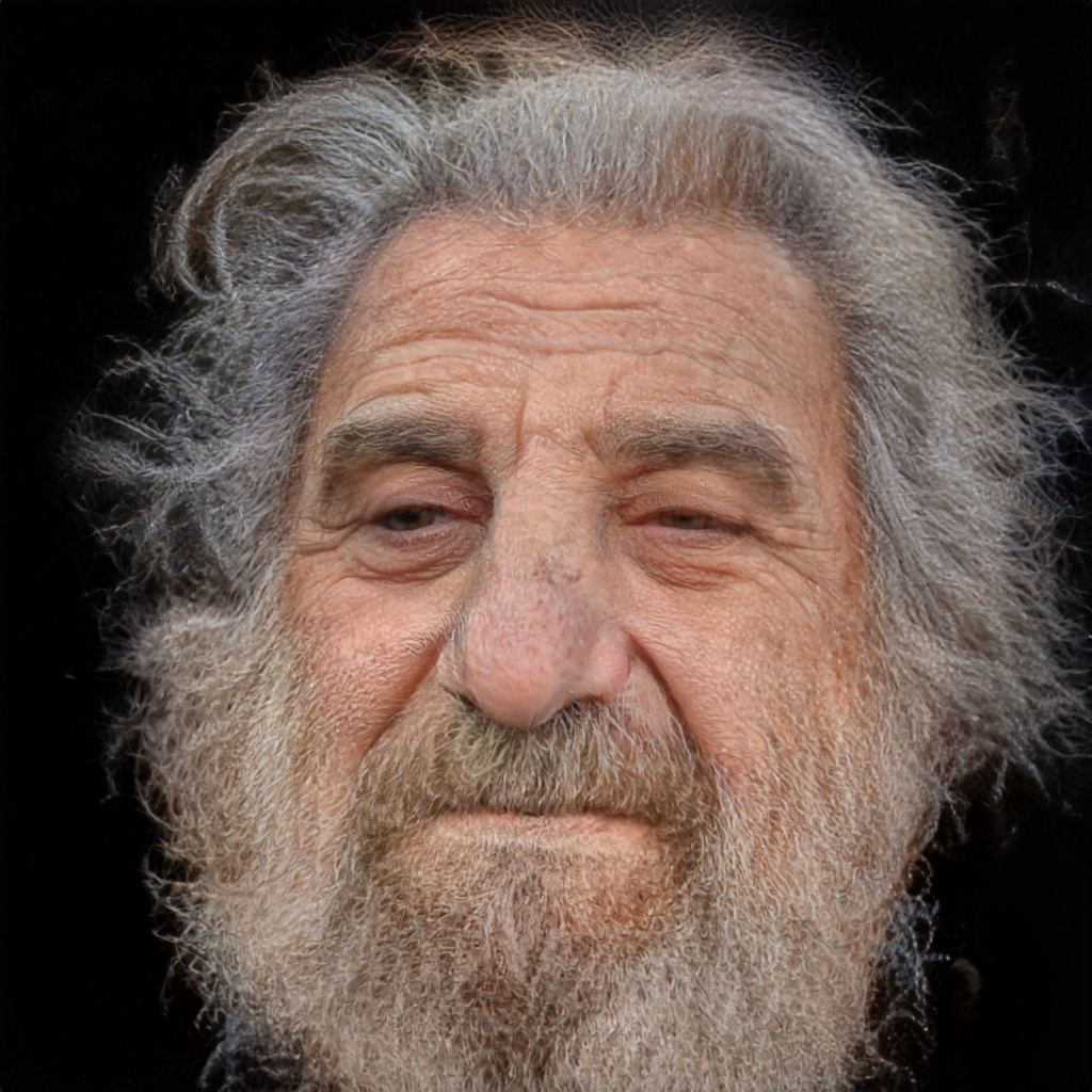
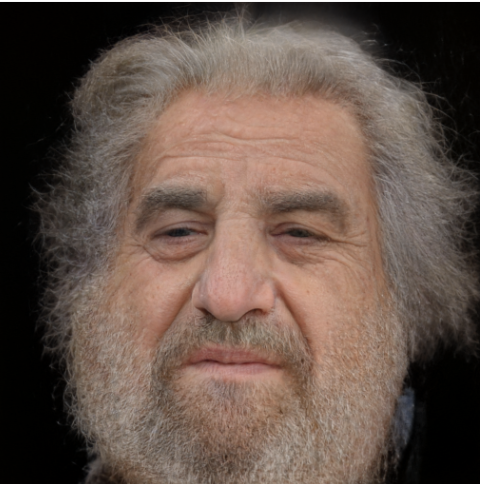
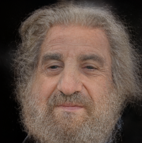
- In the next example, the antique image has many features (many wrinkles, glasses, and noisy background). The contrast and brightness are also a bit low. These might
be a few reasons for failure. The modern photo is very different from the original image.
Original Old Image
Reconstructed Image
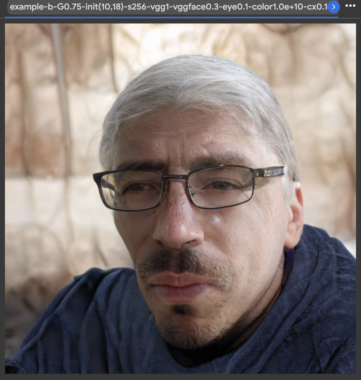
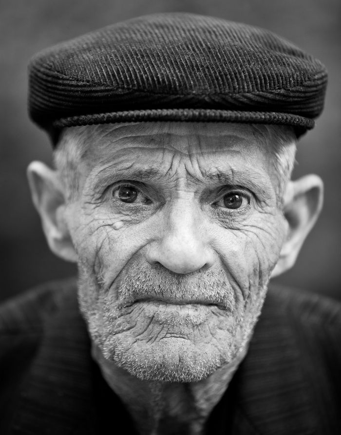
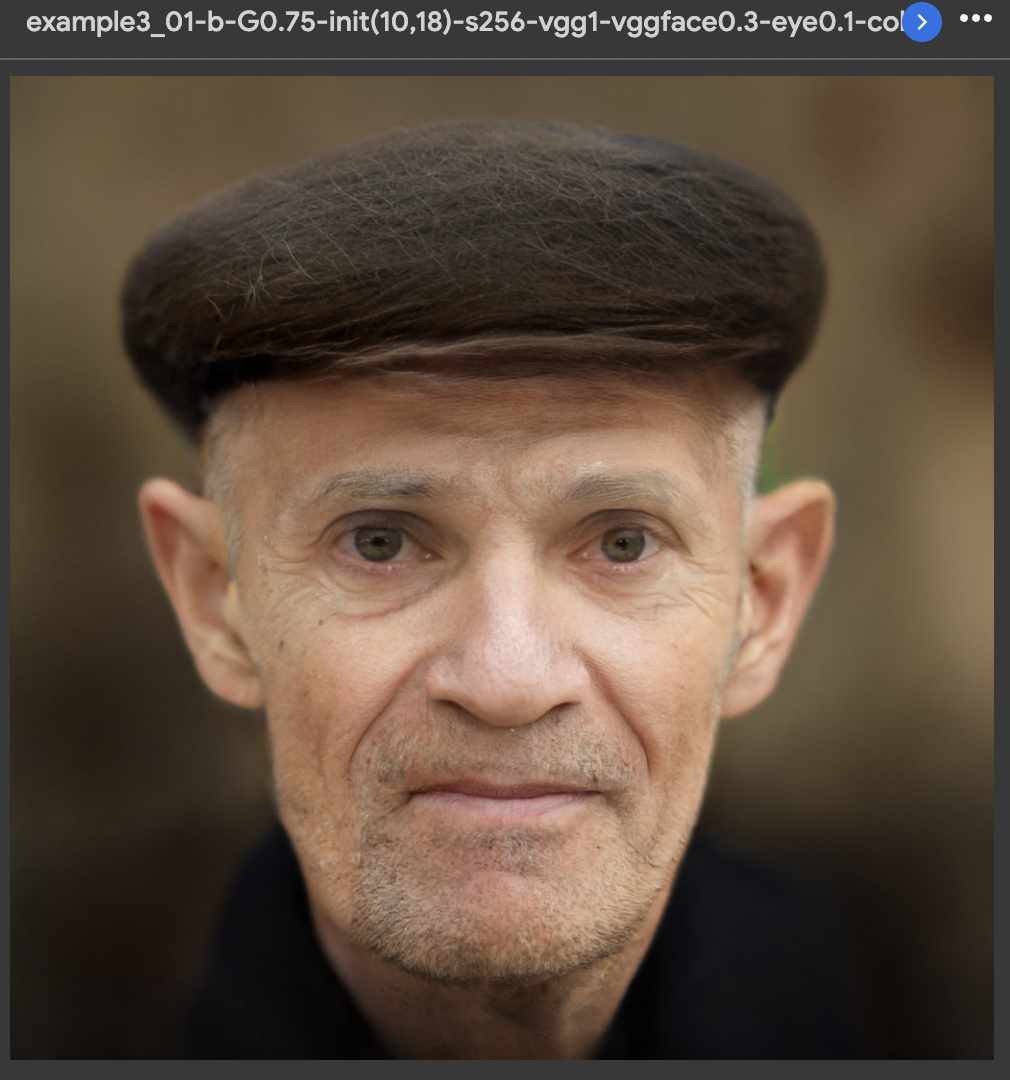
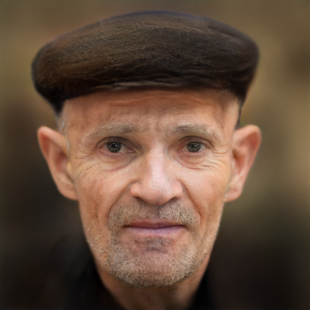
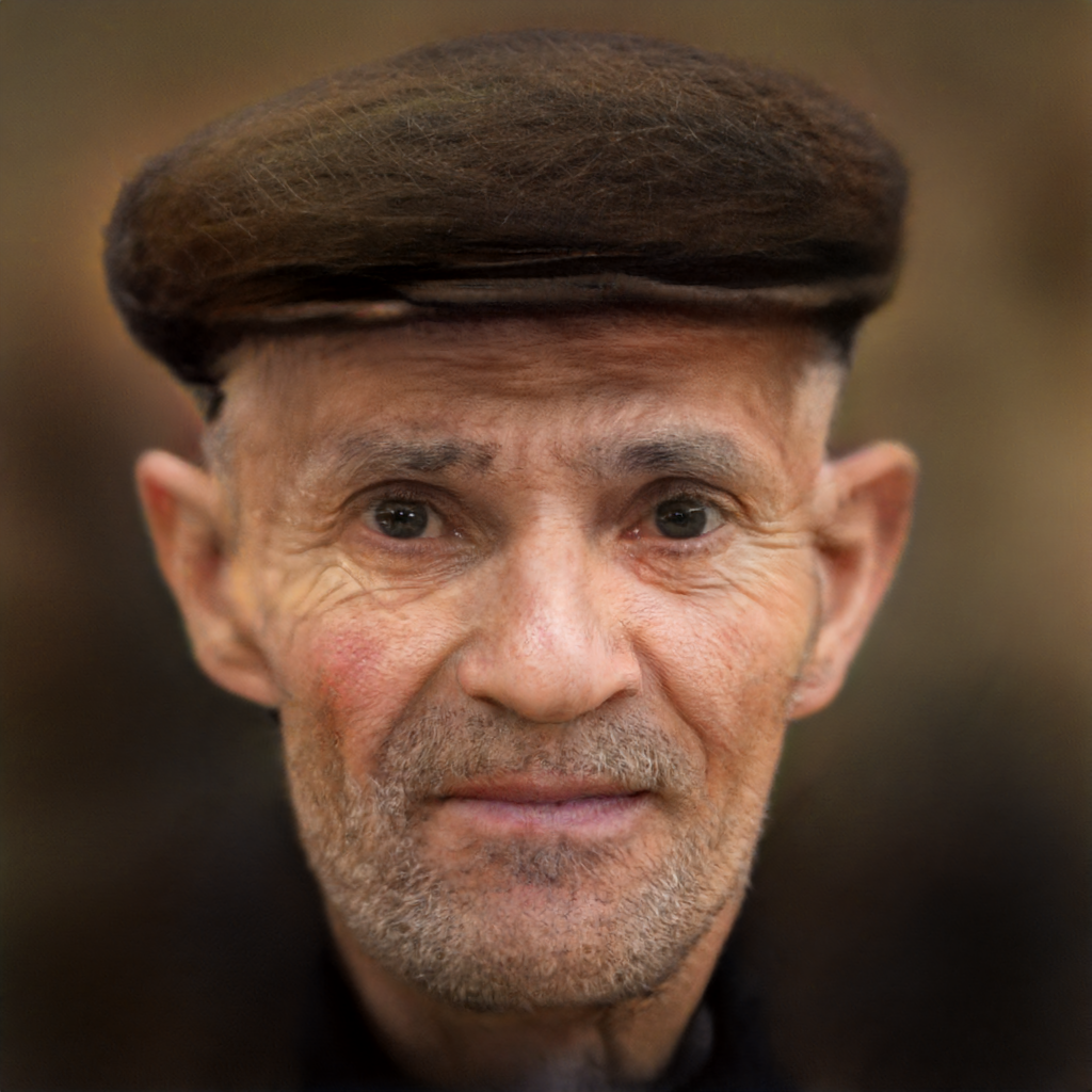
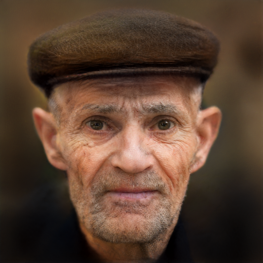
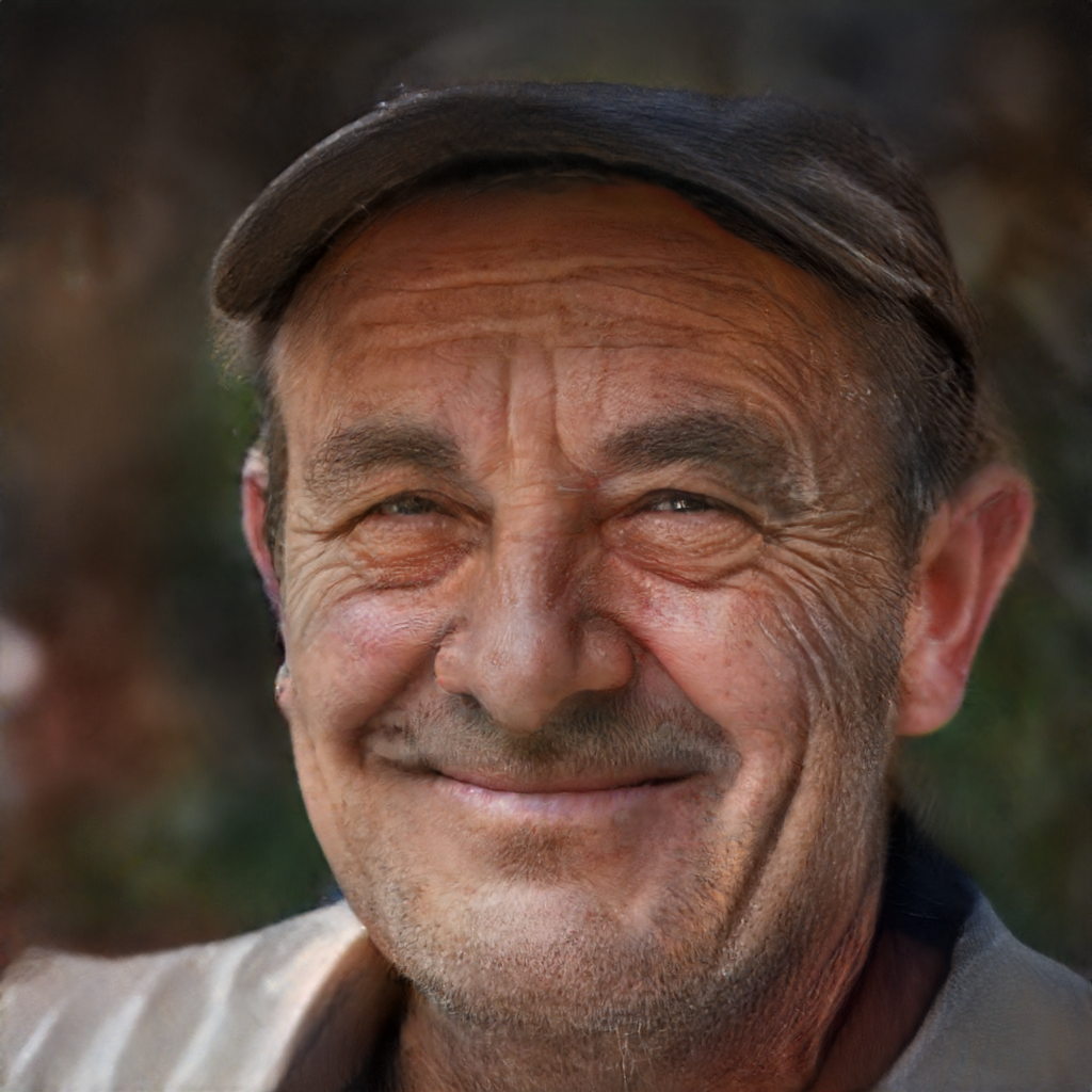
- Here, the main issue is the artifact existing in the antique photo. The hat worn by the man is translated into hair in the modern photo. The texture is also like hair.
This might be because of the shape of the hat. This is an important failure case we focus on.
Original Old Image
Reconstructed Image
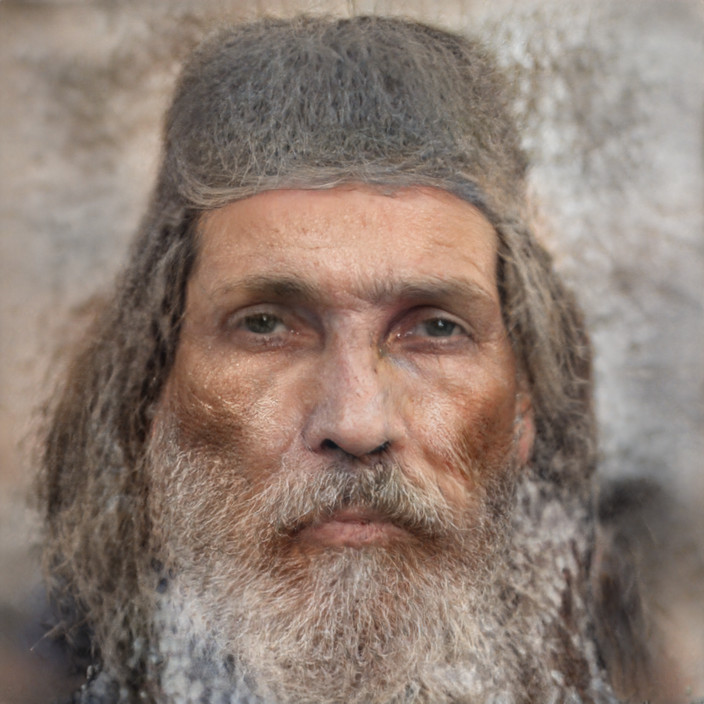
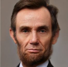
- This is an example of a subtle failure. In the antique photo, the man's hair is merging with the background since it is a light one. The man actually has scattered
hair strands. However, in the modern photo, it looks like the man has dense hair, especially on the right side. This is a misrepresentation of the antique photo.
Original Old Image
Reconstructed Image
Perceptual Loss: Using L2 Loss instead of L1 Loss
An important component of the Image Reconstruction Loss is the Perceptual Loss. In the base implementation of the
paper Time Travel Rephotography, L1 Loss is used
in the perceptual loss component. But as we saw in the failure cases, certain fine grained details are not well preserved.
There is a loss in the fine details such as the wrinkles and the skin textures which does not make the reconstruction look
accurate. In order to improve this aspect, we experiment with L2 Loss in the reconstruction and see that the final
reconstructed image that is of better qaulity and the finer details are preserved better.
L1 Loss can be defined as follows:
$$L1 Loss Function = \frac{\sum_{i=1}^{n} \left | y_{true} - y_{pred} \right |}{n} $$
Similarly we can define the L2 Loss function as follows:
$$L2 Loss Function = \frac{\sum_{i=1}^{n} \left ( y_{true} - y_{pred} \right )^{2}}{n}$$
In L1 Loss we take the mean absolute difference while in case of L2 Loss we take the mean squared error.
Both these loss functions are used commonly when it comes to image synthesis tasks and for reconstruction
purposes. The L2 loss is more sensitive to outliers than the L1 loss, meaning that it gives more weight to large errors.
This can be useful in situations where we want to penalize large errors more severely.
In our experimentation we saw that L2 Loss gave better attention to detail than L1 loss did. The use of L2 Loss
certainly provided us an improvement over using L1 Loss.
Let us take a look at few examples below.
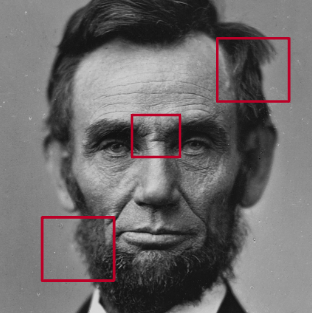
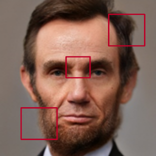
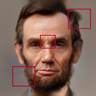
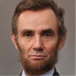
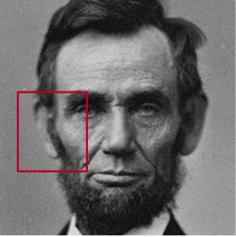
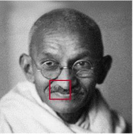
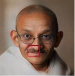
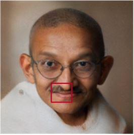
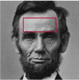
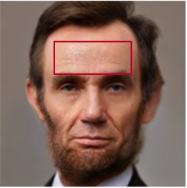
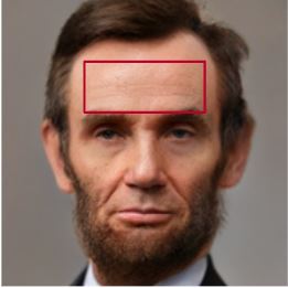
In this first example, let us concentrate on the areas demarcated by the red rectangles. If you compare the
content within the red rectangles for the original image, the image generated with L1 Loss and the image generated with L2 loss,
we see that details with L2 loss are much more finer and sharper and better preserved generally during the reconstruction.
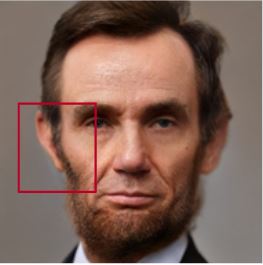
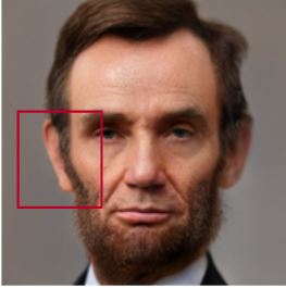
As you can see, the hair details and the beard details are much more sharper when L2 Loss is used rather than
L1 Loss. Additionally the texture in the wrinkles specifically between the eyebrows and the forehead is much better
preserved than when L1 Loss was used. Thus we can say that L2 loss certainly provided an improvement over the L1 Loss.
Original Old Image
Image Reconstructed with L1 Loss
Image Reconstructed with L2 Loss
A few more examples are shown below in order to demonstrate that L2 Loss generalises well to other images as well and this is not a one of case of improvement. The examples are as shown below.
Original Old Image
Image Reconstructed with L1 Loss
Image Reconstructed with L2 Loss
Original Old Image
Image Reconstructed with L1 Loss
Image Reconstructed with L2 Loss

Original Old Image
Image Reconstructed with L1 Loss
Image Reconstructed with L2 Loss
Original Old Image
Image Reconstructed with L1 Loss
Image Reconstructed with L2 Loss
As we can see from all the above examples, L2 Loss has clearly provided a better result overall than L1 Loss. This is one improvement we found out during the course of experimentation for this project.
Preprocess Image with Attention Based GAN
When we analyzed the shortcomings of the current approach we noticed that certain artifacts in the image such as
the accessories a person was wearing were not clear in the generated image. In order to tackle this problem we decided to
experiment with an Attention Based GAN as a preprocessing step.
In conventional GANs, the generator produces an image by taking a random noise vector as input and
transforming it using a number of convolutional layers and upsampling. The discriminator then assesses
the created image and determines whether it is authentic or phony by comparing it to the original.
In an attention-based GAN, the generator architecture includes a self-attention mechanism that enables the
generator to deliberately concentrate on key areas of the image as it is being created. A learnable attention
map that is created from the intermediate feature maps of the generator is used to implement the self-attention
mechanism. The feature maps are then weighted using this attention map, giving the crucial areas of the image
greater attention. This is the primary reason we decided to experiment with attention based GANs for the
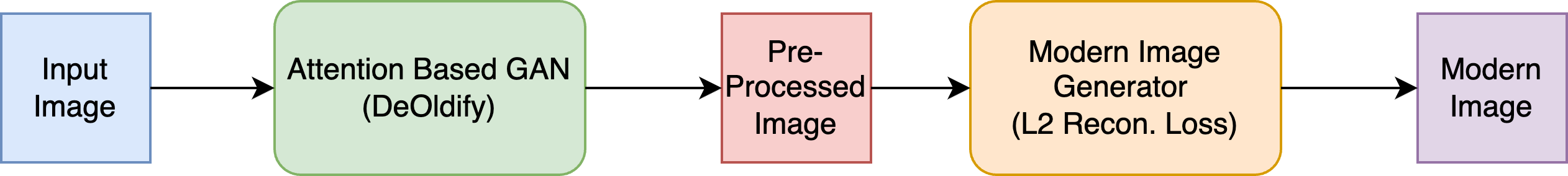
preprocessing step. In our preprocesing step we use the DeOldify pipeline and this preprocessed image is passed as
input to the modified reconstruction pipeline that involves the L2 loss in the reconstruction Loss instead of the L1 Loss. The entire pipeline is as shown below:
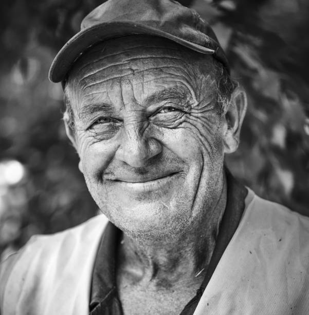
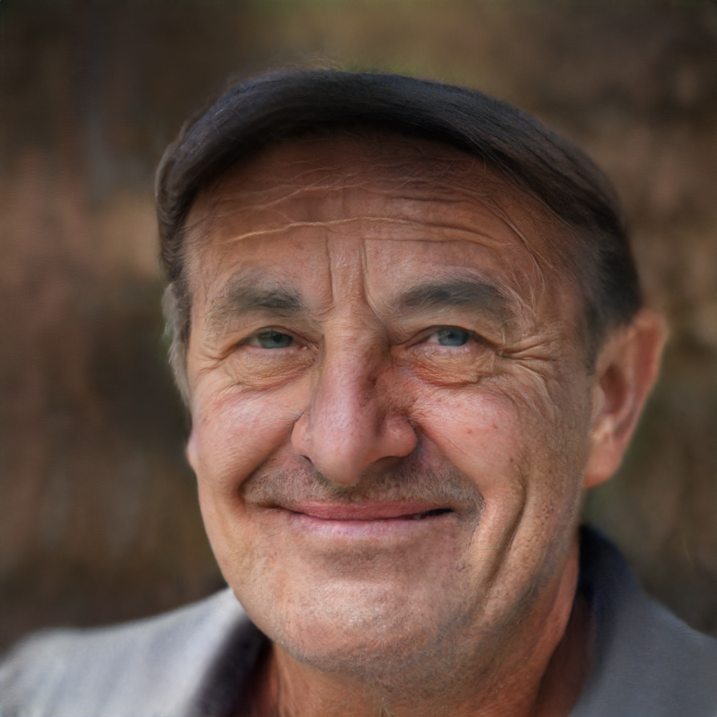
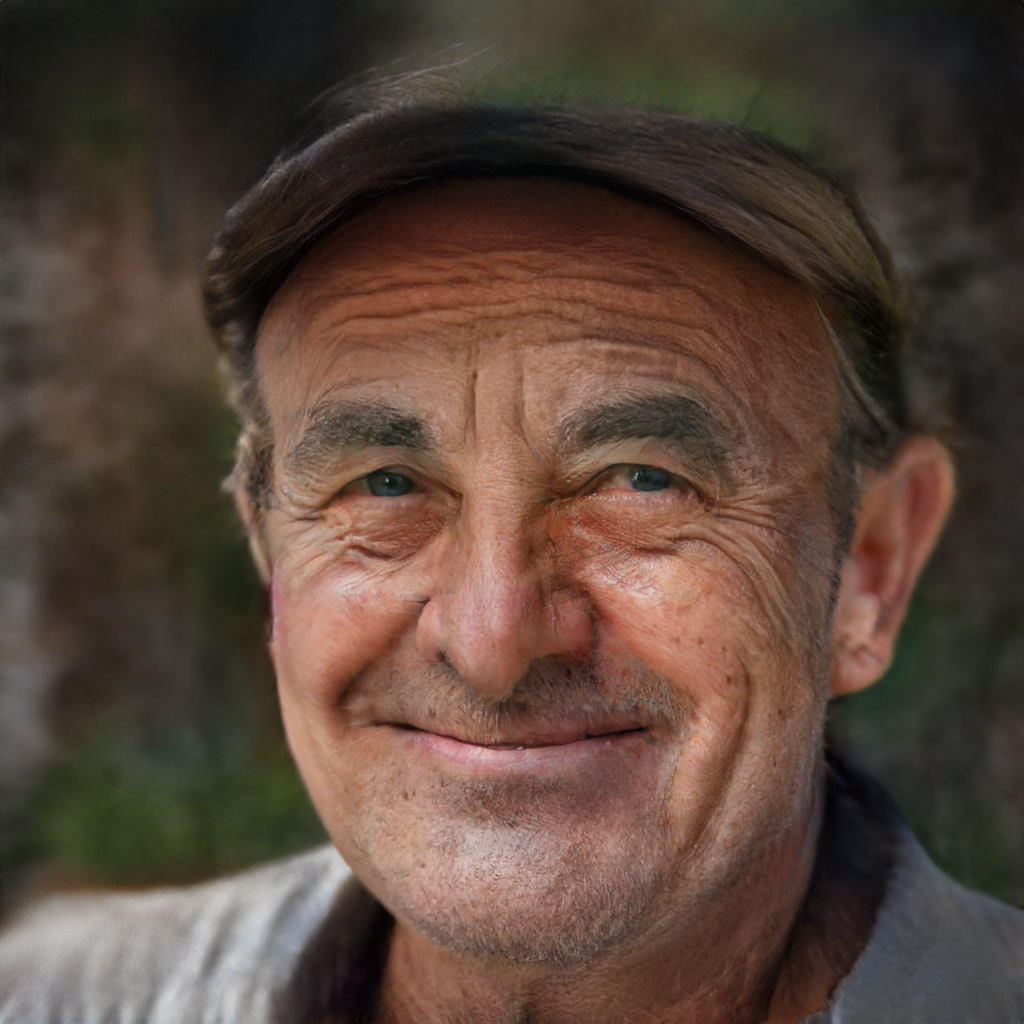
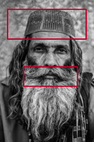
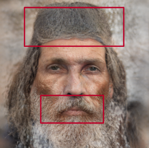
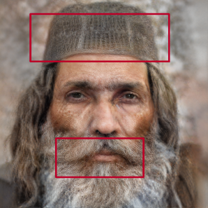
Let us now look at the a specific case where there is drastic improvement in the structure and the sharpness of the
artifiacts such as the cap and the specific beard shape when the preprocessing is performed before passing the
preprocessed image through the reconstruction pipeline. In the given example below notice the areas within the
red rectangles. When we analyze this example, we see that the structure of the cap is much better preserved
when the preprocessing is done on the image. The chequered pattern in the hat is more clearly preserved in the reconstructed
image. Additionally when we look at the structure of the moustache, we see that the overall shape and sharpness of the
moustache is better preserved overall. Hence, the preprocessing pipeline made out of the Attention-Based GAN certainly
improved the quality of the regenerated image.
Original Old Image
Image Reconstructed with L2 Loss
Preprocessed Image Reconstructed with L2 Loss
In the below example it can seen how the wrinkles become more accurate and finer when the preprocessing is done rather then when there is no preprocessing done.
Original Old Image
Image Reconstructed with L2 Loss
Preprocessed Image Reconstructed with L2 Loss
In the below example, again we can see how the wrinkles are more accurate and also the hair pattern is clearly much more accurate in comparison to not doing the preprocessing. Hence we can see that preprocessing the image clearly provides an update here as well.
Original Old Image
Image Reconstructed with L2 Loss
Preprocessed Image Reconstructed with L2 Loss
In the example below, both the wrinkles and the hat that the man is wearing become more clear when the processing is done. Without the preprocesing it seemed like the hat had the texture of hair but when the preprocessed image is used, the hat texture more closely resembles the input image. Furthermore, the wrinkles are also much more well defined than when no preprocessing was performed. Once again an improvement is seen in case of this image as well.
Original Old Image
Image Reconstructed with L2 Loss
Preprocessed Image Reconstructed with L2 Loss
Finally in the example below we can see how the wrinkles are better preserved and also the shape of the eyes is preserved better when the image is preprocessed rather than when there is no preprocessing that is performed. Overall all these examples showcase that preprocesing does improve the quality of the final reconstructed image.
Original Old Image
Image Reconstructed with L2 Loss
Preprocessed Image Reconstructed with L2 Loss
Color Transfer Loss: Using Huber Loss instead of Smooth L1 Loss
In this particular proposal, we try to use Huber Loss instead of Smooth L1 Loss in order to see
whether modifying the loss function in this way would improve the colors in the generated image or not. Though
Huber Loss and Smooth L1 Loss are quite similar, there are subtle differences which need to be discussed. Let us first look
at the formulae for both Huber Loss and Smooth L1 Loss.
Smooth L1 Loss is explained as the following:
$$ l\left (x, y \right ) = L = \left \{ l_{1}, ... ,l_{n} \right \}^{T}
\\
\\
l_{n} = \begin{cases}
0.5\left ( x_{n} - y_{n} \right )^{2} / beta & if \left | x_{n} - y_{n} \right | < beta\\
\left | x_{n} - y_{n} \right | - 0.5 * beta & ,otherwise\\
\end{cases}
$$
Huber Loss is explained as the following:
$$
l\left (x, y \right ) = L = \left \{ l_{1}, ... ,l_{n} \right \}^{T}
\\
\\
\\
l_{n} = \begin{cases}
0.5\left ( x_{n} - y_{n} \right )^{2} & if \left | x_{n} - y_{n} \right | < delta\\
delta * \left (\left | x_{n} - y_{n} \right | - 0.5 * delta \right ) & ,otherwise\\
\end{cases}
$$
Smooth L1 Loss is quadratic for small errors and linear for large errors. That said, it behaves in a manner
similar to MSE loss for small errors but it becomes less sensitive to outliers than MSE loss when the errors
are large.
On the other hand, Huber Loss is a compromise between MSE Loss and the Mean Absolute Error Loss (MAE) loss.
For small errors, Huber Loss behaves like MSE loss, while for large errors, it behaves like MAE loss.
This makes Huber Loss less sensitive to outliers than MSE loss while maintaining its differentiability.
In our case, we test with Huber Loss with delta parameter set as 0.5.
Let us take a look at an example below. As we can see from the example below, using Huber Loss over Smooth L1 loss
does not provide drastic improvement in the color of the generated image. Rather it looks a little washed out
when we make use of Huber Loss instead of Smooth L1 Loss. Hence this proposal does not provide us with a great improvement
as anticipated. From this we can conclude that it is beneficial to stick with Smooth L1 Loss instead of going
with Huber Loss.
Original Old Image
Image Reconstructed with Smooth L1 Loss
Image Reconstructed with Huber Loss
Noise Regularizer
During the image synthesis process, the global w+ style codes(StyleGAN2 network's learned style vectors) are optimized with a strong noise regularizer. By a strong noise regularizer, we mean that a regularization technique is used to control the noise input to the StyleGAN2 network. This ensures that the noise input is not carrying any significant signal and is only used to introduce controlled randomness to the image synthesis process. So, having a strong regularizer for global w+ style codes might make it hard to preserve local image details, textures, etc. We experimented with two different ways of reducing the strength of this noise regularizer. One was to just reduce the weight of the noise regularizer loss and the other way was to reduce the dimension until which the loss is calculated.
Reducing the weight
We experimented with a smaller weight for the noise regularizer loss of 5000 as opposed to the default value of 50000. But in the below images we see that this does not work and makes the reconstructed image different from the original old image. So, an alternate method to reduce the strength of the regularizer had to be found.Original Old Image
Image Reconstructed with noise regularizer weight 50000
Image Reconstructed with noise regularizer weight 5000

Reducing the pyramid resolution
The regularization is performed on noise maps at multiple resolution scales.
A pyramid structure is created by downsampling the original noise map at different resolutions, with each level
being downsampled by averaging 2x2 pixel neighborhoods and multiplying the result by 2 to maintain the expected unit variance.
The purpose of the pyramid structure is to create a set of downsampled noise maps that can be used for regularization without affecting
the actual image synthesis process. These downsampled noise maps are only used to compute the regularization loss during training and do not play a
role in the final image synthesis.
Overall, the pyramid downsampled noise maps are used to regularize the noise maps at different resolutions,
providing a smoother and more stable signal that can be used to synthesize high-quality images.
This pyramid structure is created by taking each noise map that is greater than 8x8 in size in the original method.
To reduce the strength we take noise maps with resolution just greater than 16x16 opposed to 8x8 in original method.
By this method, we were able to get improvements in preserving the basic structure of the input image in comparison to having a strong regularizer.
Original Old Image
Image Reconstructed with strong noise regularizer
Image Reconstructed with weak noise regularizer
Bicubic interpolation instead of bilinear
During resizing processes in the image synthesis process, Bilinear interpolation is used. We experimented by substituting this with Bicubic interpolation. This gave outputs with more finer details such as wrinkles preserved as shown in the image below.
This happens because Bicubic interpolation uses a larger window of neighboring pixels compared to bilinear and hence, more finer details are preserved.
Given a grid of values f(i,j), where i and j are integer indices, and a point (x,y) in between the grid points, the bilinear interpolation formula for estimating the value f(x,y) is:
f(x,y) = f(i,j)(1-u)(1-v) + f(i+1,j)u(1-v) + f(i,j+1)(1-u)v + f(i+1,j+1)uv
where i = floor(x), j = floor(y), u = x-i, and v = y-j.Given a grid of values f(i,j), where i and j are integer indices, and a point (x,y) in between the grid points, the bicubic interpolation formula for estimating the value f(x,y) is:
f(x,y) = ∑i=03 ∑j=03 ai,j * xi * yj
where a(i,j) are the coefficients of the cubic function, which are determined by solving a system of linear equations using the values of the grid points and their derivatives.Original Old Image
Image Reconstructed with bilinear interpolation
Image Reconstructed with bicubic interpolation
Conclusion and Discussion
From our efforts of improving the model in the base paper, we were able to achieve the following results -
- We were able to improve the quality of the images produced by preserving the fine features of the antique photo. This was achieved by switching to L2 loss, reducing the strength of the noise regularizer, and by using bicubic interpolation.
- We experimented with Huber loss, however could not see much change in color transfer results.
- Another major improvement we made was preprocessing input image with attention based GAN (DeOldify) to remove artifacts before generating modern image. This helped to reproduce correct images of artifacts such as hats, glasses, etc.
Future Work
In the future, we propose using the pSp (pixel2style2pixel) encoder instead of the e4e (encoder4editing) encoder. The former is said to work better than the latter when
an image with a distribution different from the training data is given during inference time. pSp encoder also helps to capture local features of the image better.
Another direction we propose to work in the future is the use of some other dataset for training. The authors of the base paper have declared that this model might
contain some bias due to the underrepresentation of certain groups while using StyleGAN2. This can be fixed by using a dataset with lesser bias. One such example is
the FairFace dataset. Retraining the model with this dataset can help reduce the bias.