Joshua Cao | Carnegie Mellon University
About Course
16-726 Learning-Based Image Synthesis / Spring 2022 is led by Professor Jun-yan Zhu, and assisted by TAs Sheng-Yu Wang and Zhi-Qiu Lin.
This course introduces machine learning methods for image and video synthesis. The objectives of synthesis research vary from modeling statistical distributions of visual data, through realistic picture-perfect recreations of the world in graphics, and all the way to providing interactive tools for artistic expression. Key machine learning algorithms will be presented, ranging from classical learning methods (e.g., nearest neighbor, PCA, Markov Random Fields) to deep learning models (e.g., ConvNets, deep generative models, such as GANs and VAEs). We will also introduce image and video forensics methods for detecting synthetic content. In this class, students will learn to build practical applications and create new visual effects using their own photos and videos.
Assigment Summary
| Topic | Abstract | Reference | |
|---|---|---|---|
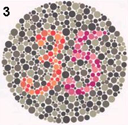
| A1 | Colorizing the Prokudin-Gorskii Photo Collection | Implement SSD, pyramid structure, USM, auto crop, contrast methods |
Dataset USM Hough Transform |
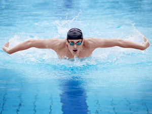
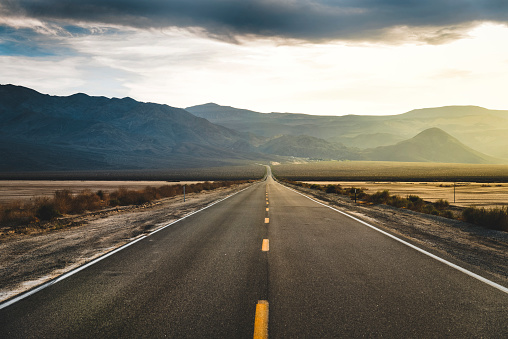
| A2 | Gradient Domain Fusion | Implement Poisson Blending, Mixed Blending, Color2Gray |
Poisson Blending |
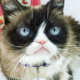
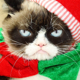
| A3 | When Cats meet GANs | Implement DCGAN, CycleGAN |
Dataset CycleGAN-pix2pix |
| A4 | Neural Style Transfer | Vgg-19, style transfer | |
| A5 | GAN Photo Editing | Inverted GAN, StyleGAN2, Interpolation, Sketch2Image |
AdaWild Dataset 256/128 Resolution Cat Dataset |
Copyright
 All datasets, teaching resources and training networks on this page are copyright by Carnegie Mellon University and published under the Creative Commons Attribution-NonCommercial-ShareAlike 4.0 International License. This means that you must attribute the work in the manner specified by the authors, you may not use this work for commercial purposes and if you alter, transform, or build upon this work, you may distribute the resulting work only under the same license.
Assignment #1
Introduction
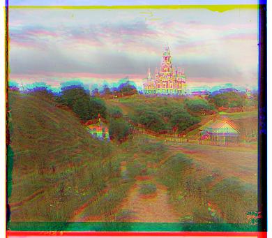
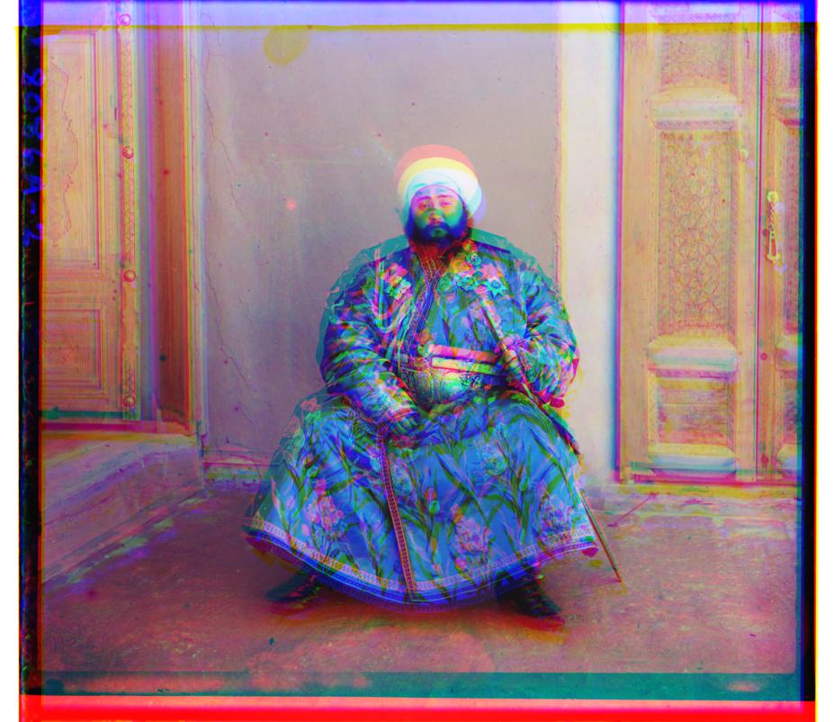
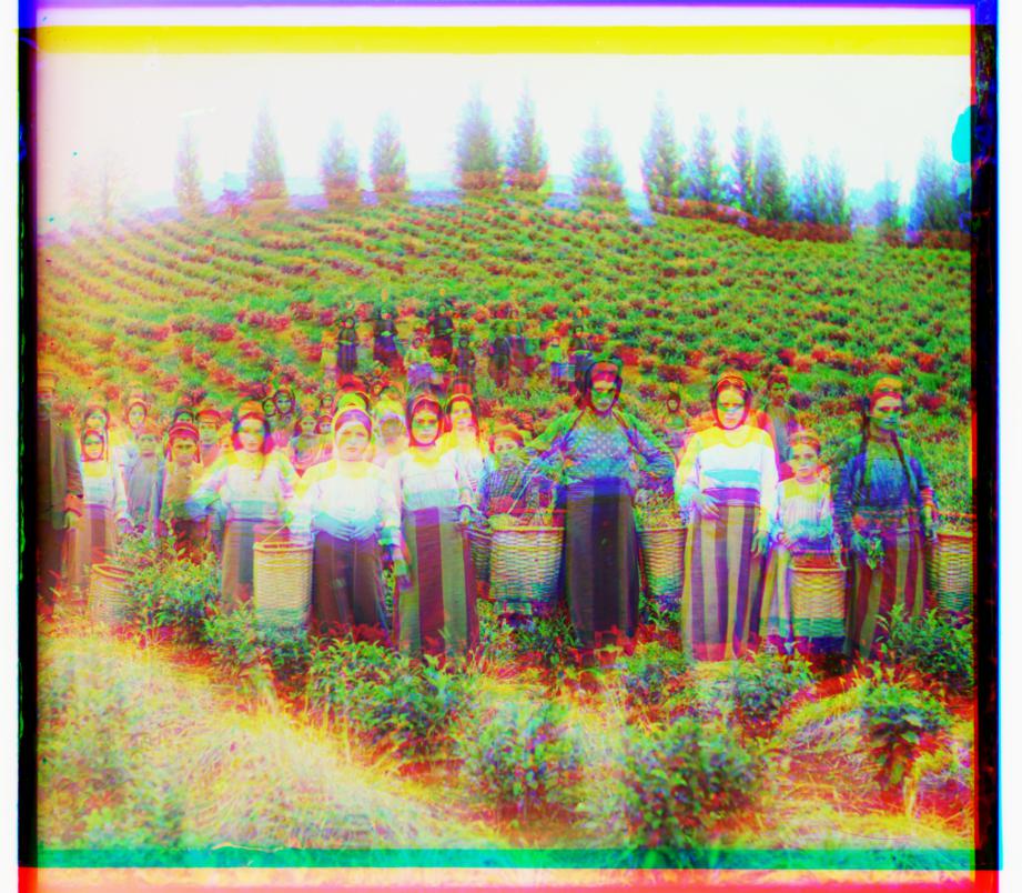
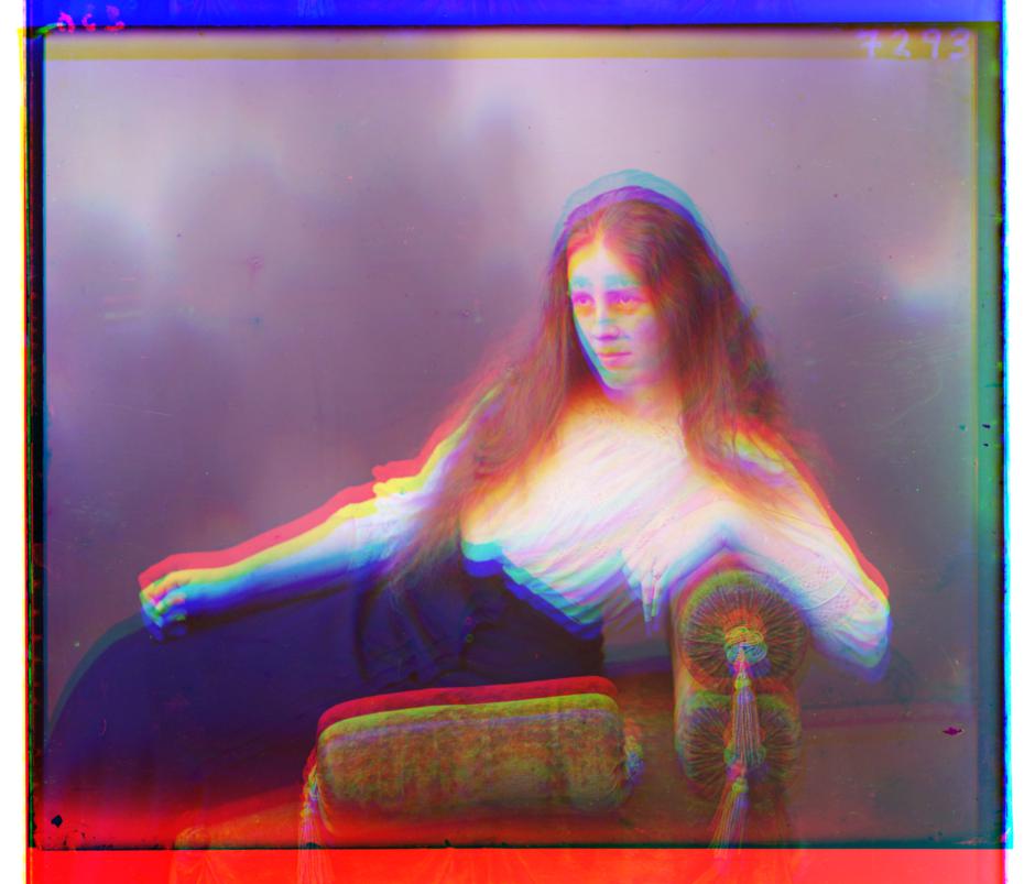
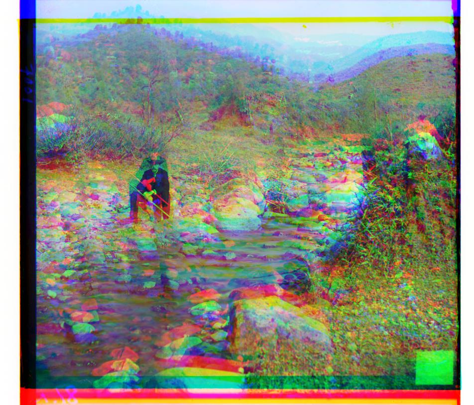
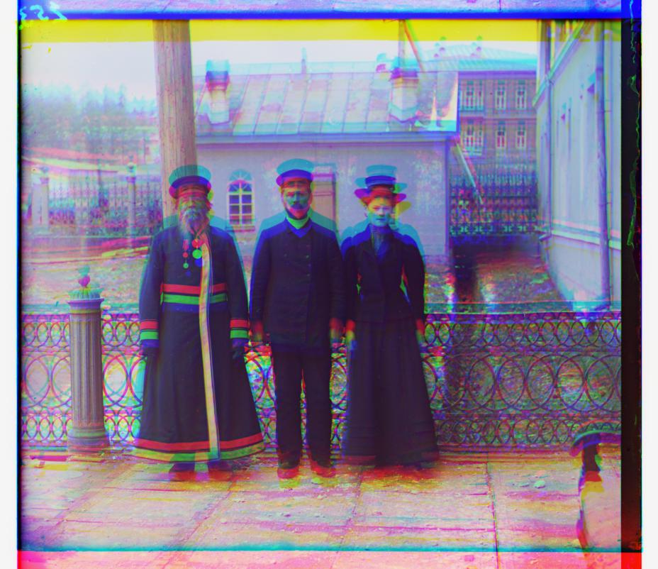
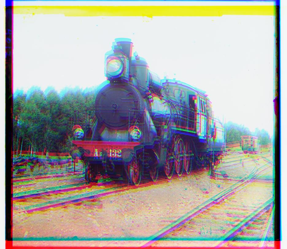
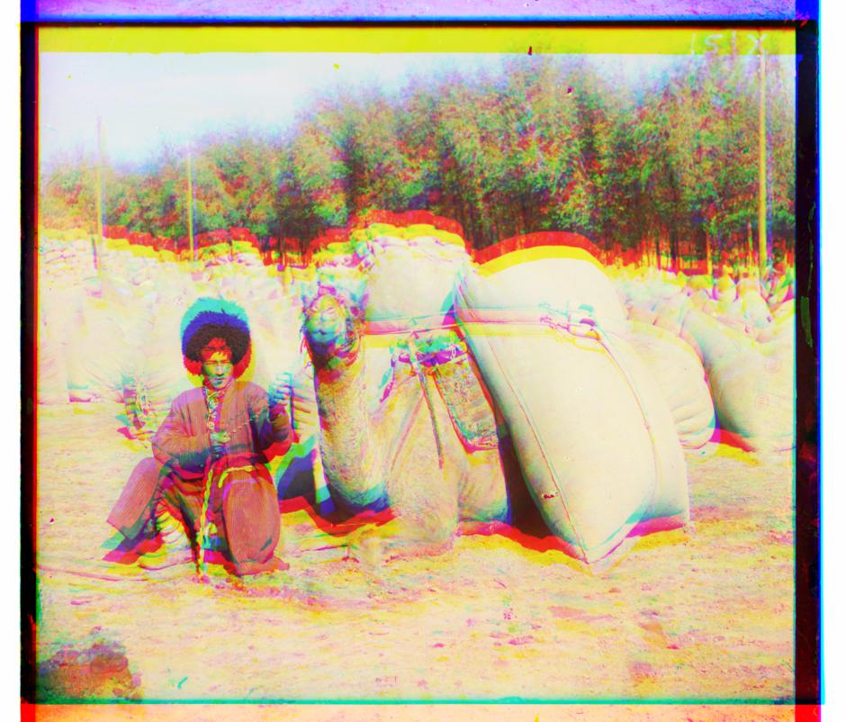
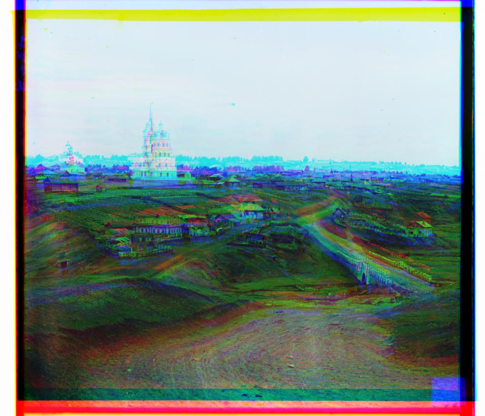
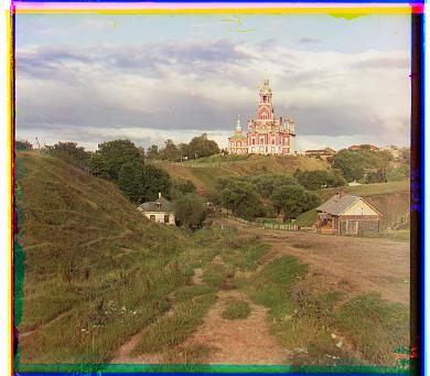
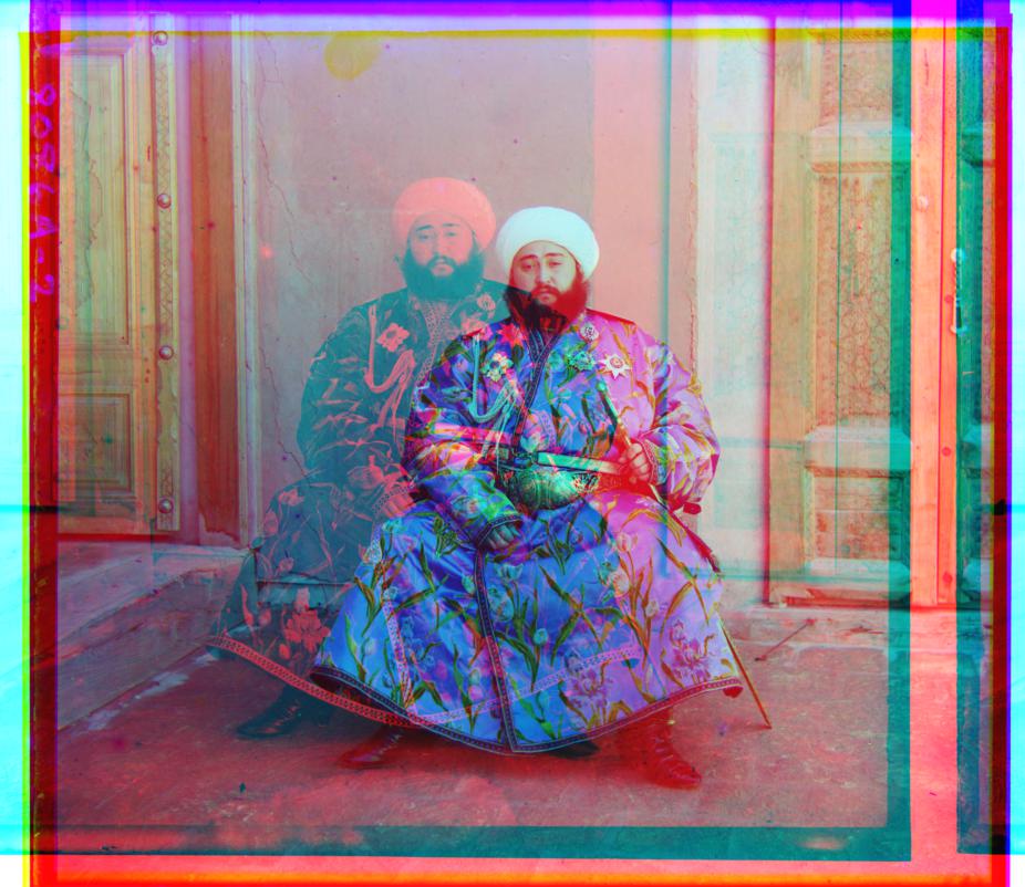
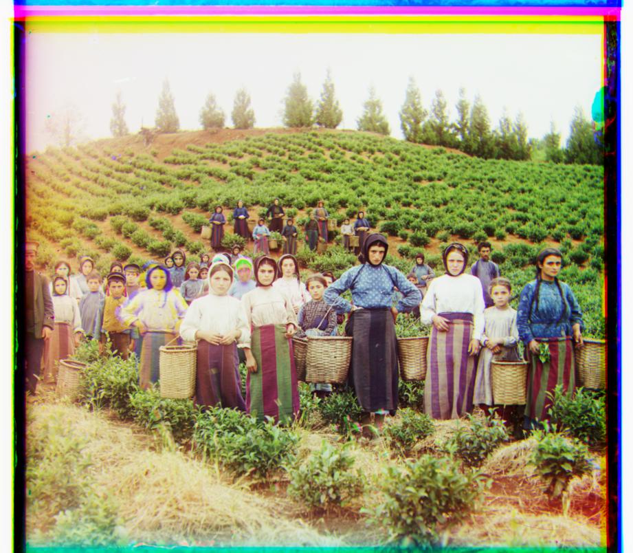
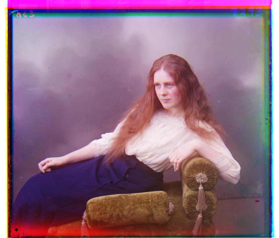
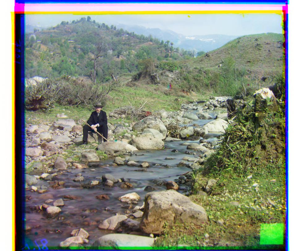
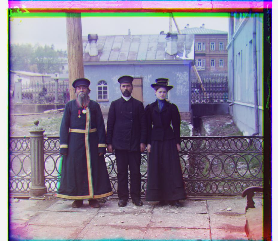
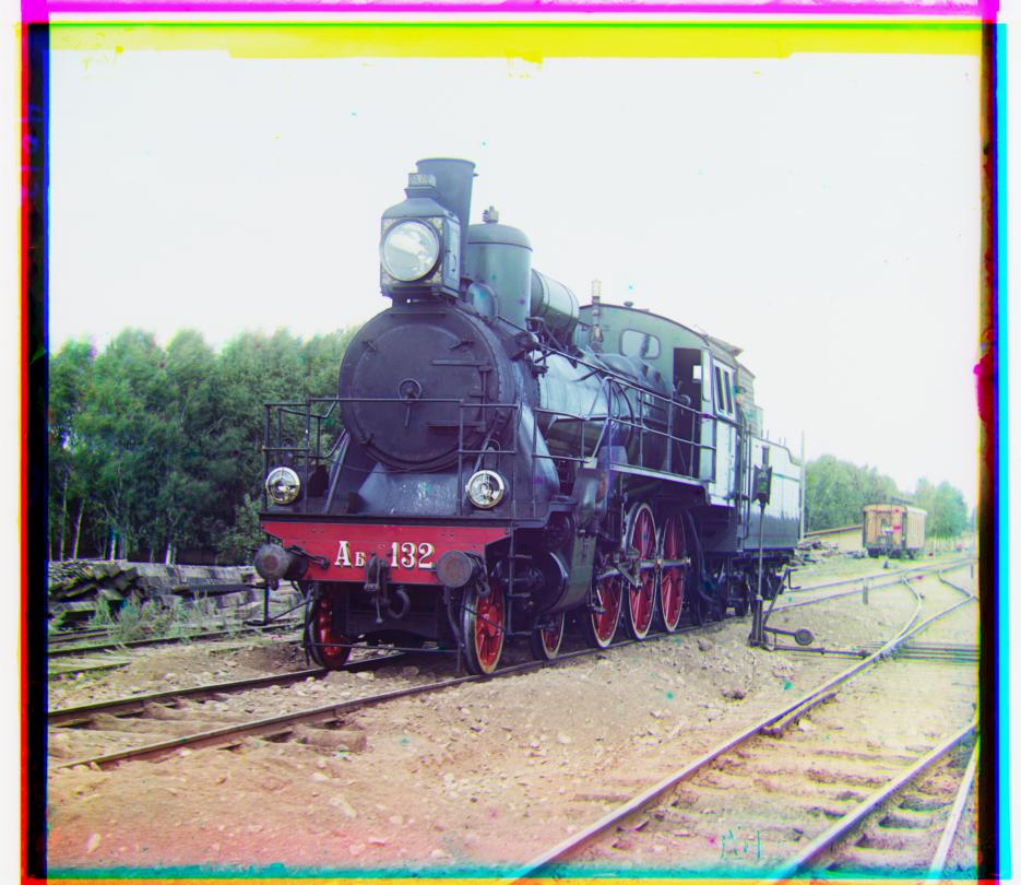
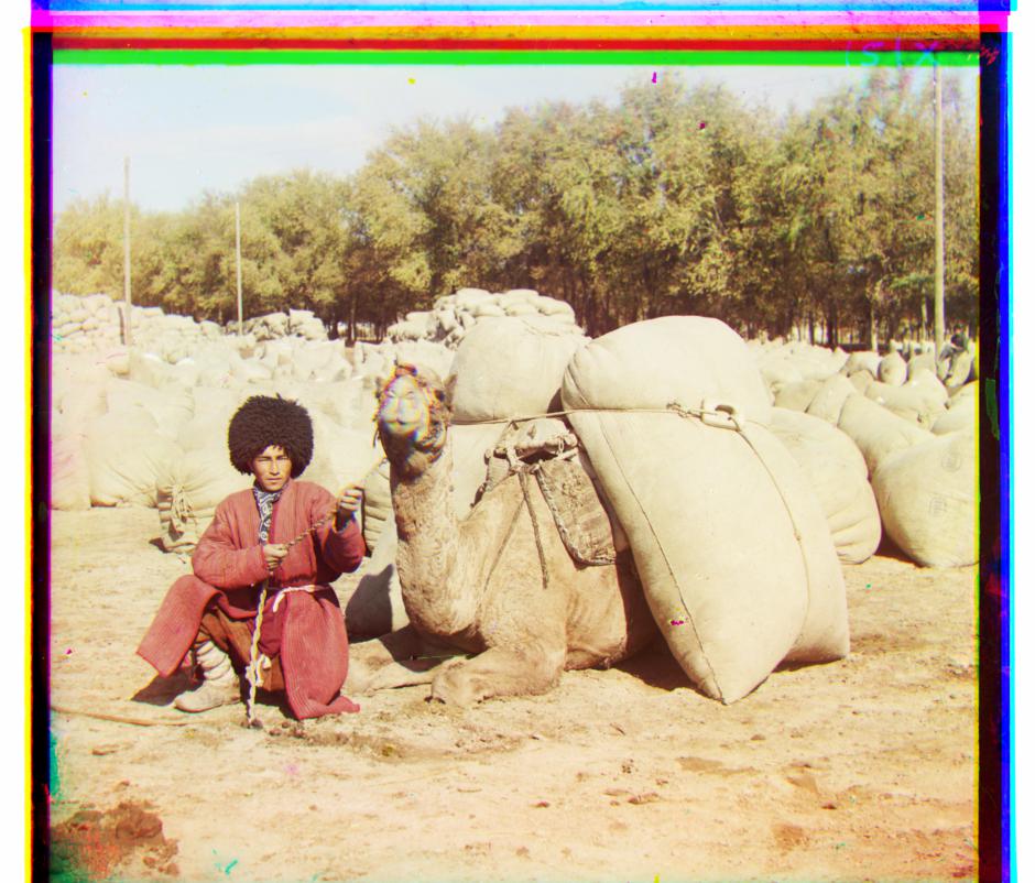
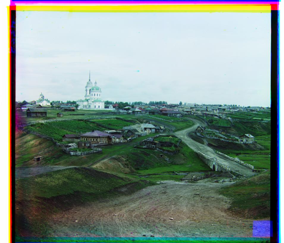
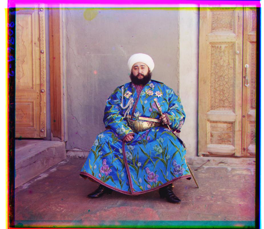
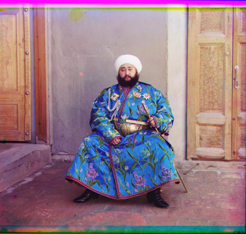
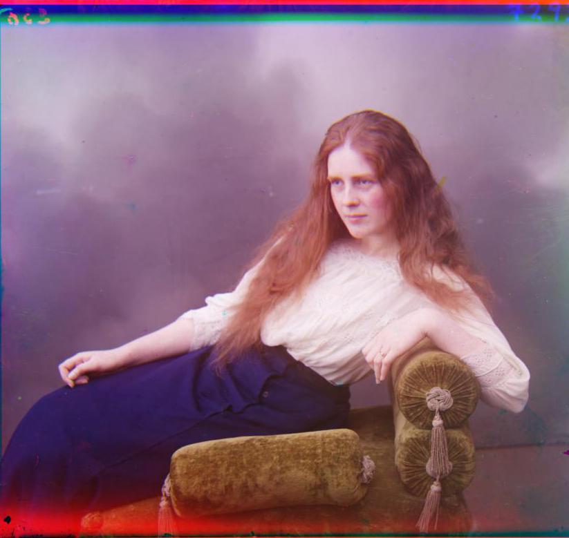
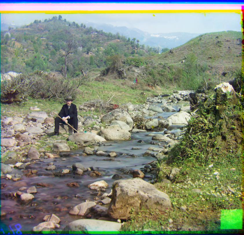
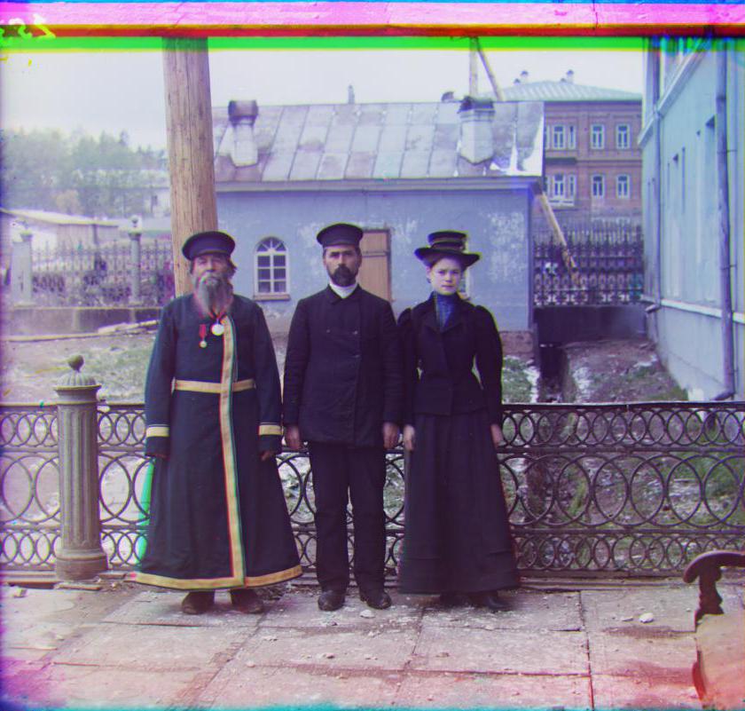
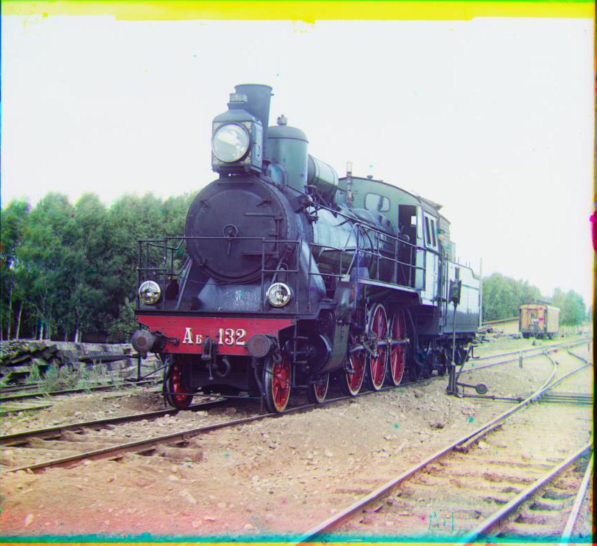
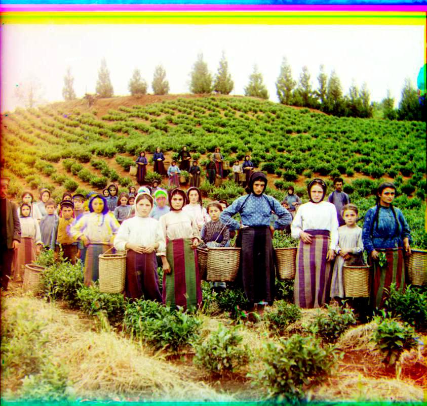
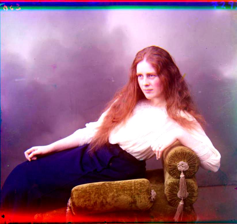
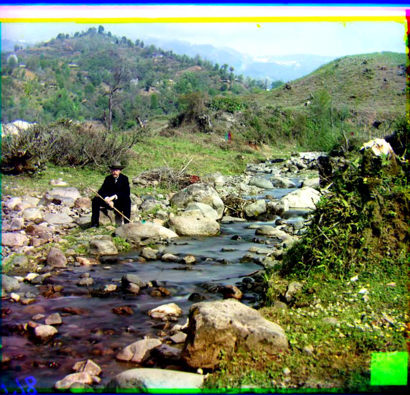
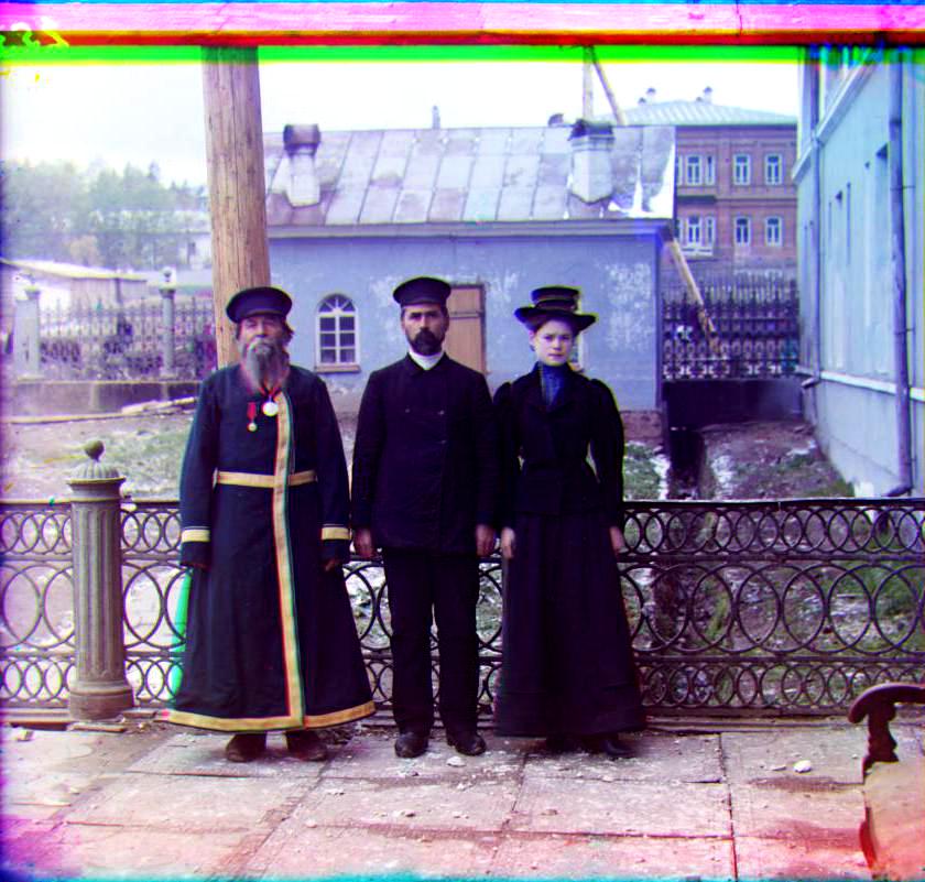
The Prokudin-Gorskii image collection from the Library of Congress is a series of glass plate negative photographs taken by Sergei Mikhailovich Prokudin-Gorskii. To view these photographs in color digitally, one must overlay the three images and display them in their respective RGB channels. However, due to the technology used to take these images, the three photos are not perfectly aligned. The goal of this project is to automatically align, clean up, and display a single color photograph from a glass plate negative.
Direct Method
Before diving into algorithms, I decide to blend R, G, B images directly and have an intuitive feeling of the tasks, which at the same time provides a reference to compare how far my algorithm can go. There are total 1 small jpeg and 9 large tiff images from the given dataset. Their direct blending goes as below:
SSD & NCC Alignment
I implement both SSD and NCC to compare the small patch's similarity for alignment, the search range is [-15,15], and the algorithm works both well on the small jpeg image as shown below. To speed up the calculation, I also cropped 20% of each side of the image to decrease calculation on the edge. However, to deal with larger image, not only the search range is not large enough, but also the calulation takes extremely long. Therefore, the pyramid structure comes to practice.
Pyramid Aligment
I use log2(min(image.shape)) to find out how many mamixmum layers the image can have, and add conditions to only apply the pyramid algorithm for images larger than 512*512, and the small image can directly use [-15,15] SSD search. For large images, my starting layer is a size around 265 pixels(2^8 as first layer), and exhaustively search till the original image size, because I realized missing final layer will give me color bias all the time(misalignment of color channel is very easy to detect even though it's just small pixels). The first implementation of my method took 180s for one image. To speed it up, I recursively decrease search region by 2 each time to shorten it to 55 seconds per iamge, because the center of search box is determined by last layer, so the deeper algorithm search, the smaller search range it requires to find the best alignment. The output is listed as below. As you can see, most of the images are aligned quite well but image like the piece of Sergei Mikhailovich Prokudin-Gorskii, work even worse than direct alignment, this is because the brightness of the images are different, therefore, I use an USM(Unsharp Mask) algorithm to fix the issue.
Extra Credits
USM Unsharp Mask
The USM algorithm is mainly to sharpen or soften the edge of images, and allows accurate SSD difference to make better alignment. The algorithm is called for each recursion in the pyramid alignment, and it first uses Gaussian Blur to blur the single channel(gray) image, and subtract it from the original image, then I take the region of difference that is larger than certain threshold and subtract them from the original image and multiple certain constant parameters. Here I use subraction because I notice certain edge needs to be softened instead of being sharpened, due to some disturbing edges stand out too much in the original image that makes SSD find the wrong alignment. The USM specifically improves the quality of this image:
Crop Image
To get rid of the borders, I mainly use two cropping method, the first one is to keep area only for all three channels have contents, and remove those blank area caused by alignment, this is implemented by retriving shift of each single channel image. But this method can't deal so well with the region that is originally black or white outside the image. Then I use a MSE(Mean Square Error) method to calculate each row and each column's error, and set up when three adjacent rows or columns all are smaller than certain threshold, it is the area should be cropped. The result shows as below:
Add Contrast
The contrast method is pretty straight-forward, I just calculate the accumulative histogram of the image, and take 5% and 95% as 0 and 255 respectively, and stretch the color value in between so that the contrast of the main image increase.
Other Dataset
I find some other similar dataset that has pretty large tiff image to test the algorithm. The result shows as below
Assignment #2
Introduction
The project explores the gradient-domain processing in the practice of image blending, tone mapping and non-photorealistic rendering. The method mainly focuses on the Poisson Blending algorithm. The tasks include primary gradient minimization, 4 neighbours based Poisson blending, mixed gradient Poisson blending and grayscale intensity preserved color2gray method. The whole project is implemented in Python.
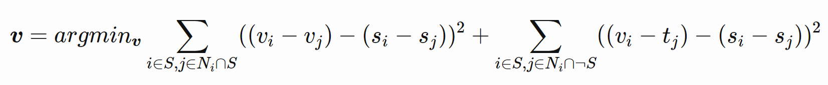
Toy Problem
The toy problem is a simplifed version of Poisson blending algorithm, therefore it helps understanding the Poisson blending a lot. The major functions are three, to calculate the gradient of x axis and y axis, and to align the left-top corner (0,0) of the image:
((v(x+1,y)−v(x,y))−(s(x+1,y)−s(x,y)))**2
((v(x,y+1)−v(x,y))−(s(x,y+1)−s(x,y)))**2
(v(1,1)−s(1,1))**2
We use the equations to loop through each pixel of the source image to construct A and b. By solving the least square form of Av=b, we can get the synthesized image v. Say the given gray image size is H by W, A's dimension is H*W by 2*H*W+1, b's dimension is H*W by 1. The result is pretty much to test if we can copy the original image, as shown below:
I implemented it in both loop method and non-loop method, the interesting thing is that with loop method, it only takes around 0.4s, whereas with the non-loop method, which is supposed to be faster in Python environment than loop, turns out to take around 10s. I think the major reason is that sparse matrix's arithmetic calculation is more expensive than directly assign value to coordinates. In the non-loop method, I mainly use lil_matrix to construct sparse matrix, and use np.roll, np.transpose to construct A matrix. Finally I decide to use the loop method for the rest of the task.
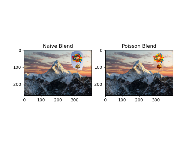
Poisson Blending
Based on toy problem's hint, Poisson Blending explores the four neighbour of each pixel, follow the equation below that v is the synthesized vector that we need to solve, s is the source image in the size of target image(but we're only interested in the masked source image), t is the target image:
In the equation, each i deals with 4 j, i.e. the same i is calculated 4 times with 4 different neighbour j. The left part considers the condition if all the neighbour of i is still inside the mask, and the right part considers the neighbour not all inside the mask. Notice the difference in code is that for the right part, tj is used to construct parameter b, whereas for the left part, vj is used to construct parameter A.
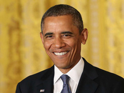
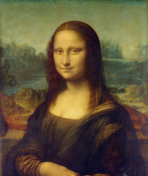
Also, the given image now has RGB, 3 channels, therefore we need to calculate each channel separately. When I implemented it, I consider that A matrix is always the same for 3 channels, but b are different for each channel, therefore I only calculate A once and b 3 times to speed up the algorithm. What's more, since the we only need to generate image from the maksed source image's coordinate, I only loop through this area to speed up. And finally I merged three v together to get new RGB image. The average speed is related to the image size, to deal with the given example of 130x107(source image) and 250x333(taget image), it generally takes around 20s.
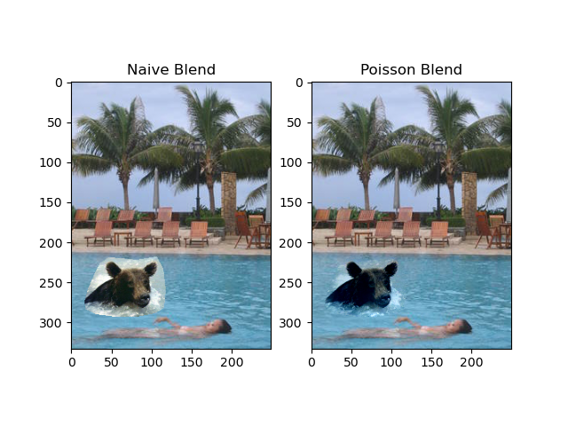
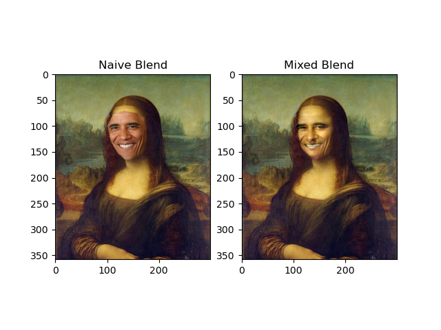
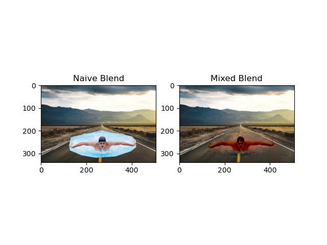
However, the naive Poisson Blending has some issue to deal with blending the image seamlessly, which is because only considering the source neighbour is not enough for strong difference of target and source images. As you can see the image below, the inner part of the ballon house is little blur and not blended so well with the background. Therefore, we need to implement Mixed Blending.

Extra Credits
Mixed Gradients
Mixed gradients is actually pretty straight forward based on Poisson Blending, we just add one condition that instead calculating the gradient of source image s, we compare the gradient of s and gradient of t, and take the larger one so that it can better blend when the difference of source and target image are large. The comparison of the same image can be seen as below(The left is blendered without Mixed gradients.):

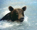
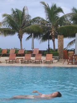
The given example of bear and pool is below:
There are some more generated blending images:
And there is a failure case where the colorful Patrix can't blend so well with the gray-scale like moon image:
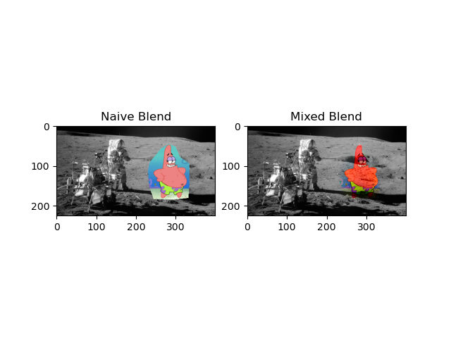
This is mainly because there is upper limitation of the blending algorithm to adjust the color, if the source image and target image have too large difference, the algorithm will reach its limitation to find the solution that best approximate the least square function.
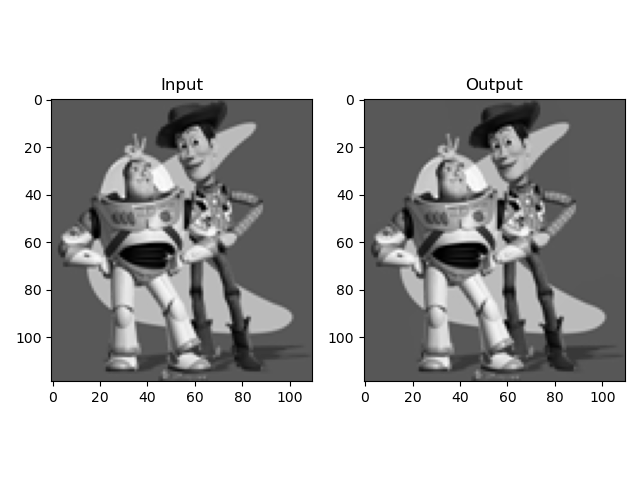
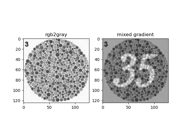
Color2Gray
The Color2Gray method first turns RGB image to the HSV color space, and only consider the S and V channels to represent the color contrast and intensity respectively. In this way, we can keep the color contrast of rgb image and preserve the grayscale intensity at the same time. The algorithm runs similar to the Mixed Gradient where source and target image are S and V. The result is shown as below:
Assignment #3
Introduction
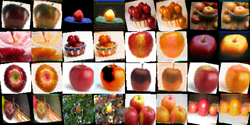
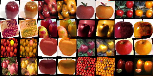
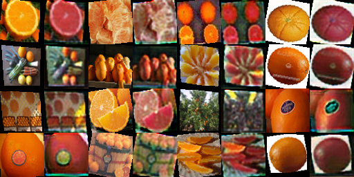
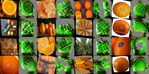
This project implements two famous GAN architecture: DCGAN and CycleGAN. It is programmed in Pytorch, the major code includes the build-up of discriminator and generator neural network, loss function, forward and backward propagations. It also explores different methods that help GAN generate better results, such as Data Agumentation, Differentiable Augmentation, variance of different lose functions, variance of different discriminators, and implemented in different dataset to check the robustness fo the network.
Part I: Deep Convulotional GAN
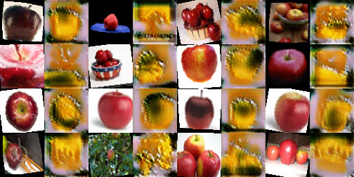
Implement Data Augmentation
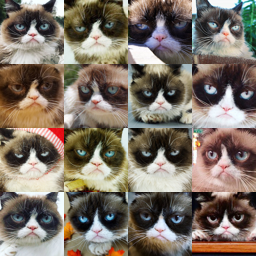
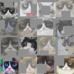
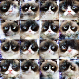
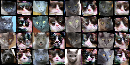
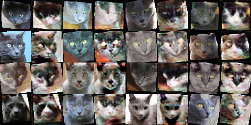
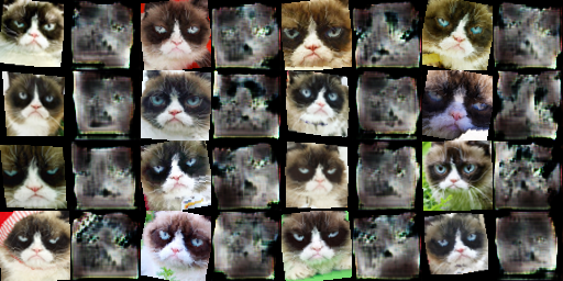
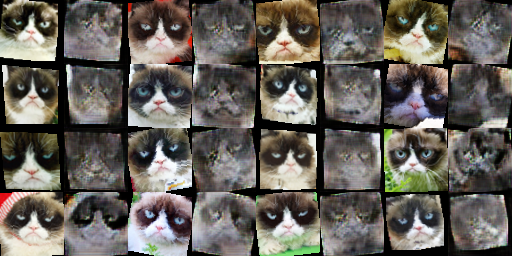
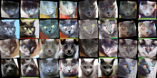
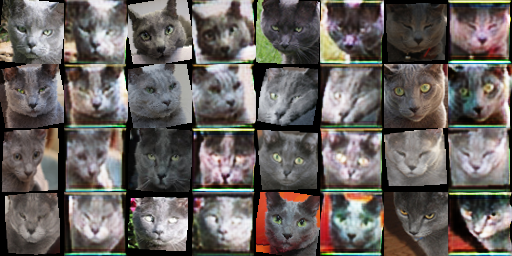
In Pytorch, data augmentation is invoked each time when iterated through the mini-batch, the purpose of the data augmentation is add variance to the dataset, which is especially useful when the dataset is small or each sample of the data are too similar. For example, in this DCGAN training, we only have 204 images as dataset. I mainly use the Resize + RandomCrop, RandomHorizontalFlip, RandomRotation(10 angles) to generate augmentation. The example of orignal dataset and augmented dataset, and GAN generated sample by different dataset can be see here:
The Discriminator
The discriminator in this DCGAN is a convolutional neural network with the following architecture:
According to the formula (N-F+2P)/S + 1 = M(We don't consider dilation here), where N is the input number of channels, M is the output number of channels, S is stride, P is padding, F is size of filter/kernel, since we want N=2M, and we use filter size of 4, stride of 2, we can calculate that padding P is 1. Besides, I use softmax for the output layer, and later on squared mean difference for loss function, since this Discriminator is a classification problem, the softmax-loss combination is a generally good choice.
The Generator
The generator in this DCGAN is a convolutional neural network with the following architecture:
In the generator neural network, I use transposed convolution with a filter, size of 4, stride of 1 and padding of 0 for the very first layer that from 100x1x1 input to 256x4x4 output. And the rest layer all are upsampling of 2, with a filter, size of 3, stride of 1 and padding of 1 to satisfy the condition that output dimension is the 2 times of input dimension. And the reason why the first layer is a transposed convolution is that it has better performance than direct upsampling for noise.
The Training Loop
The training loop including loss function and backpropagation is as straight forward as image below:
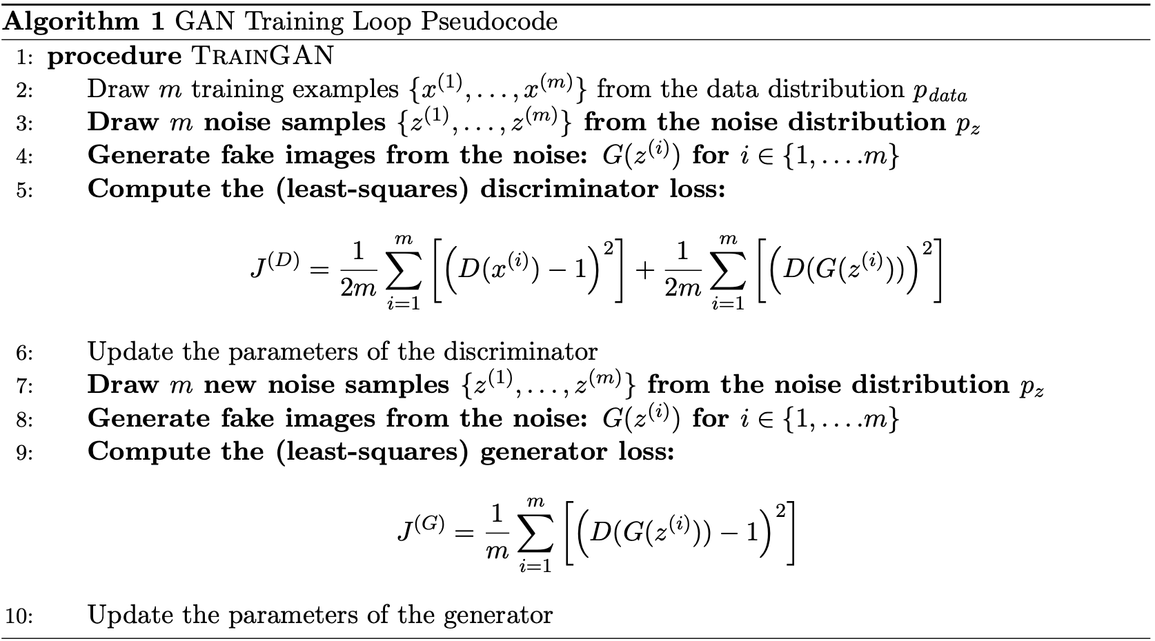
One thing to notice is that we normally first do the back propagation to update the gradients and weights of discriminator, then do the generator, this is because the loss function first goes back to discriminator then to the generator. To better train generator's weight, we prefer the gradient and weights of discriminator is static than dynamic.
Similarly, when training the discriminator, we don't want to update the gradient all the way back to generator, therefore we have to set no_grad_up for the fake_image that is generated from generator and fed to discriminator. In my case, I use torch.detach() function.
The Differentiable Augmentation
The Differentiable Augmentation method is meant to process data during the training process, it can slow down the training but can significantly improve the output's performance. And it's shown as below:
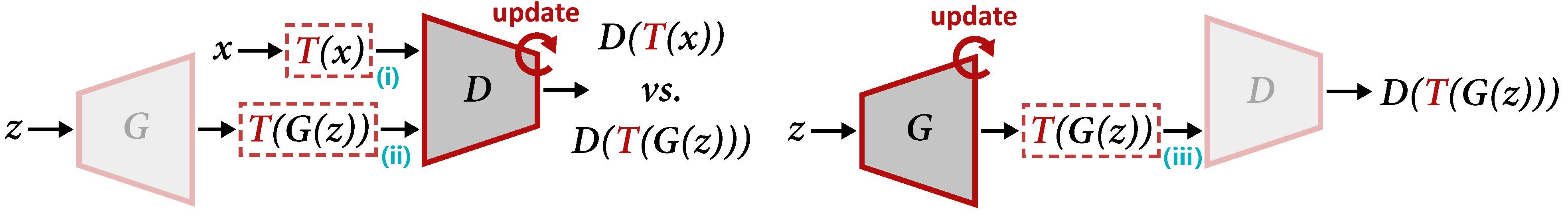
I apply differentiable augmentation to all the generator generated fake images and real images during the training process.
Results
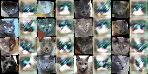
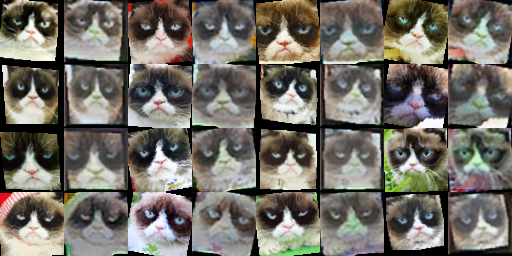
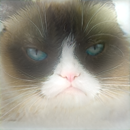
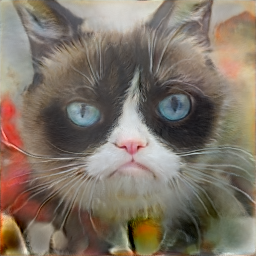
After the training with learning rate = 0.0002, beta1 = 0.5, beta2 = 0.999, epoch = 500, batch_size = 16, I get the results as below. From left to right, they are generated image with basic data augmentation, with basic and differentiable data augmentation, with deluxe data augmentation, and with deluxe and differentiable data augmentation.
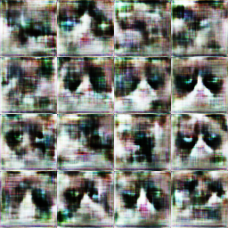
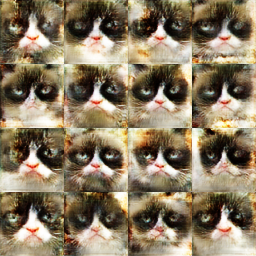
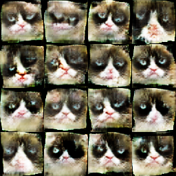
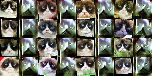
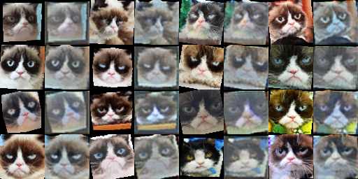
The result is interesting. It's obvious the basic method has a clumzy, hard to tell cat generation. And the differentiable method clearly has some color intensity and white balance shift, it actually proves the ability of this method to increase the robustness towards the RGB color intensity, and generate a more general color tone results, also it has a better recognition in the shape of cat. The deluxe result has a better detail than the differential method. And finally, the mix of deluxe and differential method is hard to tell if it's better than a single method, because some of the generation has both good detail and color tone but some are more blur or distorted, but if we only want one best result from a group of samples, this mix method definitely works better than either of the single method.
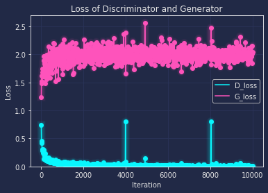
Similarly to the order above, I also draw the loss curve along with every 200 iteration as below:
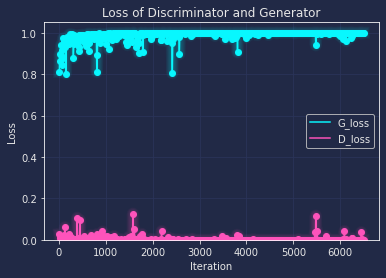
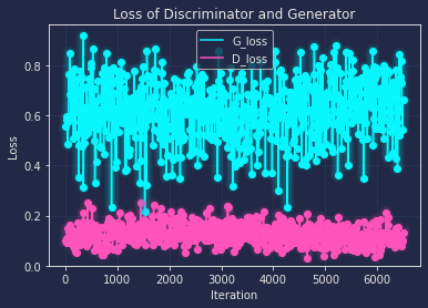
From the loss curve, we can tell that the base and deluxe both have the trend to overfitting after the training, though dexule has a relatively better loss(where G and D both are close to 0.5), and with the help of differentiable augmentation, the loss is more close to the ideal value, which means the network has a better robust performance on general data.
Part II: CycleGAN
The Dual Generator
The generator of CycleGAN is a convolutional neural network with the following architecture:
In the generator neural network, there are two generator for X->Y and Y->X, they are symmetric in input and output, and their architecture are identical in this project. The filter size is the same as in DCGAN, refer to them in convolution and upconvolution layer respectively. And one major difference is the ResnetBlock, which is used 3 times here, which aims to make sure characteristics of the output image (e.g., the shapes of objects) do not differ too much from the input. One major difference of this generator from the one of DCGAN is that its input is not noise anymore but an image.
The PatchDiscriminator
A major difference of this PatchDiscriminator from the Discriminator of DCGAN is that its output is a 4x4 patch instead of a loss value, which means the output layer doesn't require a softmax function anymore, and the rest are pretty much the same.
The Training Loop
The training loop including loss function and backpropagation is as straight forward as image below:
The major loss function and pipeline are similar to DCGAN, except for that for generator, since we have two generators, and we want to train them at the same time, so we add both X->Y and Y->X loss here; And for the discriminator, it goes the same way to train the loss from fake images generated from X->Y and Y->X.
The Cycle Consistency
The cycle consistency is like the soul part of the CycleGAN from my own experience of experiment, it aims to
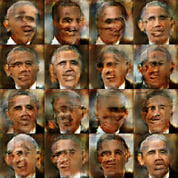
The CycleGAN Experiments
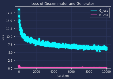
My training for CycleGAN follows the learning rate = 0.0002, beta1 = 0.5, beta2 = 0.999, batch_size = 16 same as DCGAN, and I always use the Differentiable Augmentation since it helps increase robustness towards the RGB intensity and other factors. I first start by testing the CycleGAN with epoch = 1000, with and without cycle consistency, and the results are(Left side are without cycle, right side are with cycle; up side are X->Y, down side are Y->X):
It's clearly that 1000 epoch is not enough to get a good output, but from the basic shape of it, and the loss function below, we can tell that the general direction is good to extend the epoch.(Left without cycle, right with cyckle) And we can tell that the cycle consistency has a slightly better output.
Next I extend the epoch to 10000, and train the CycleGAN with two datasets, also I made comparison that with and without cycle consistency, patchDiscriminator and DCDiscriminator. The result are listed below:(Left is patch+cycle, middle is patch no cycle, right is dc+cycle)
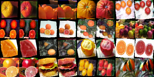
By observing the results above, we can see that without cycle consistency(middle column), the generated results have weird color, unclear shape. And for the DCDiscriminator(right column) and PatchDiscriminator(left column), they both achieve a relatively good result that generated fake image assembles the real image a lot. And they both have this color re-mapping effect, by comparison, I think the PatchDiscriminator has a slightly stronger color shift in all interested regions. It means that PatchDiscriminator can perform better pattern rematch effect.
Bonus
Extra dataset
I choose one dataset from https://data-efficient-gans.mit.edu/datasets/ to apply to DCGAN, the output is like:
Assignment #4
Introduction
Neural Style Transfer is a vgg-19 based nueral network, utlizes regression method MSE for loss function, and LBFGS for input image(noise) optimization. It only uses the feature extraction part of vgg-19, and only for evaluation purpose(no gradient optimizaiton for these layers), instead, the optimizaiton happens in the loss function and input(two ends). And the loss function consists of two parts, content loss and style loss, we'll implement them separately first, and then combine them together with assigned weights.
Part 1: Content Reconstruction
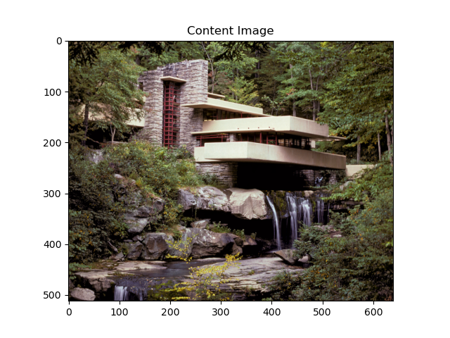
Content reconstruction mainly tries to regress a noise to an input content image, so that noise can gradually resemble the content image, therefore, the loss function is a straightforward MSE, and in implementaion, because we don't want to update vgg-19, the detach is added at the end of vgg-19. I first try content loss for each single layer and have a general direciton of how the noise approxiate the content image under the impact of different dept of neural layer's feature. Here is the result with input of a dancing.jpeg:
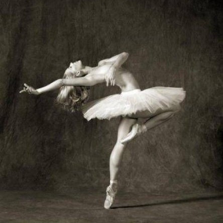
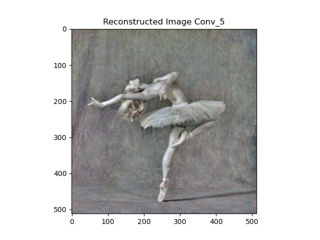
Compared with the input content image, it's not hard to tell that the shallower layer the content loss is put, the loser the noise ends up to the content image. I think the deeper layer output is more interesting, so I tried several conbinations for the deep layers from 3-5. The results are below:
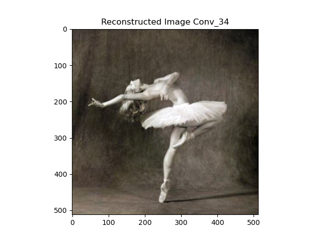
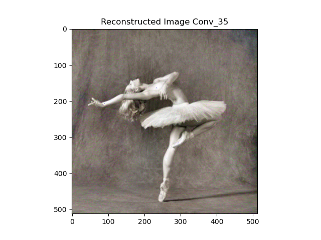
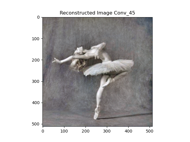
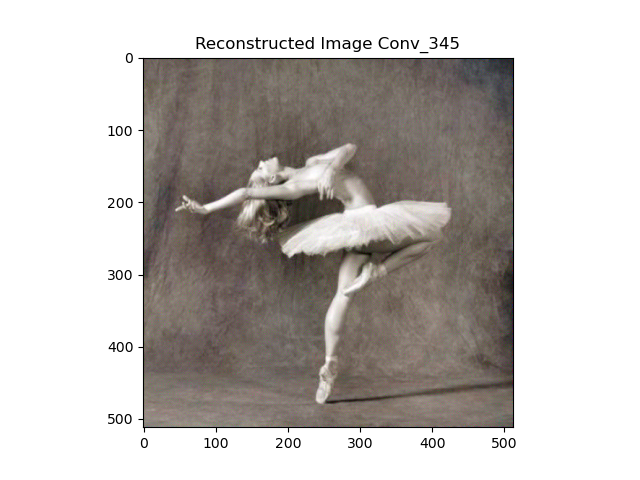
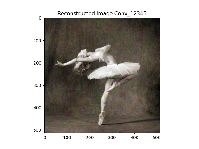
First look at the last image, we can tell if we calculate content loss in every layer, the result is pretty much like single layer 34 and single layer 3, which means that shallow layer's loss has dominated the output. And 35, 45, 345 are pretty much close to layer 4 with different color saturation, the difference is trivial and the choice if more like a style preference. I personally like the faint style, so I simply choose to apply content loss to layer 4, because it seems easier with blend with style if the content image has low saturaion. And I use two different white noise to generate the content image, the results are very much the same.
.png)
Part 2: Texture Synthesis
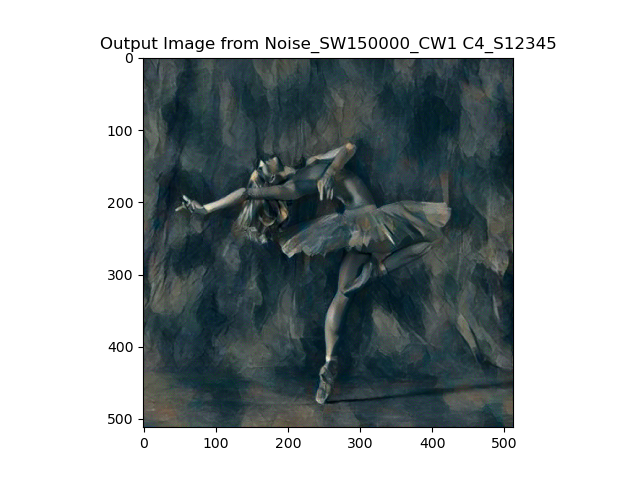
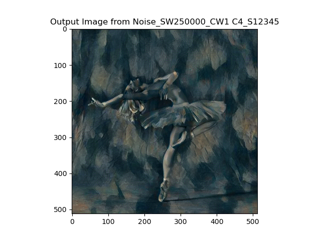
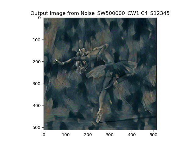
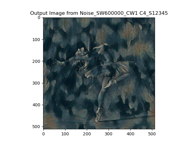
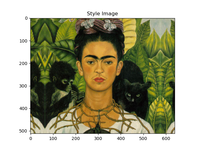
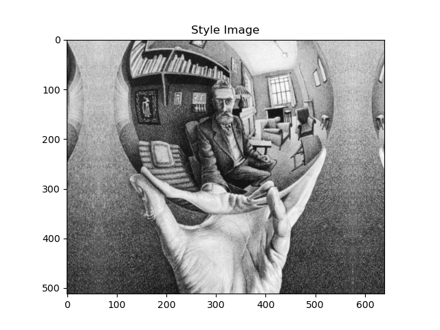
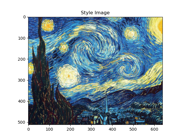
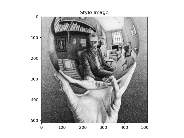
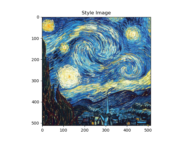
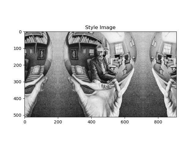
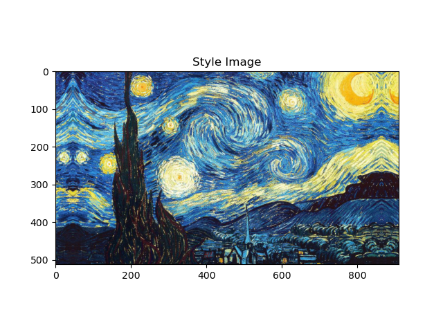
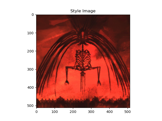
Style synthesis is pretty much the same as content structure, except for that the output of vgg-19 is processed with gram_matrix and then calculated the MSE loss. Similarly, I first try different single layer with picasso.jpeg:
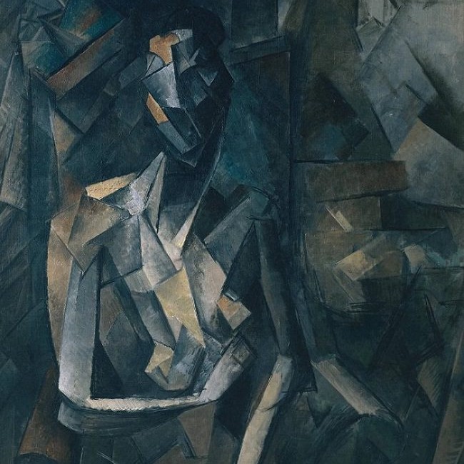
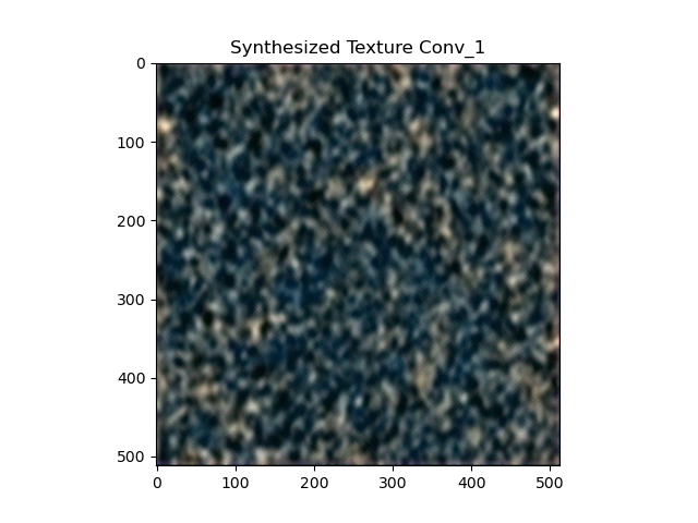
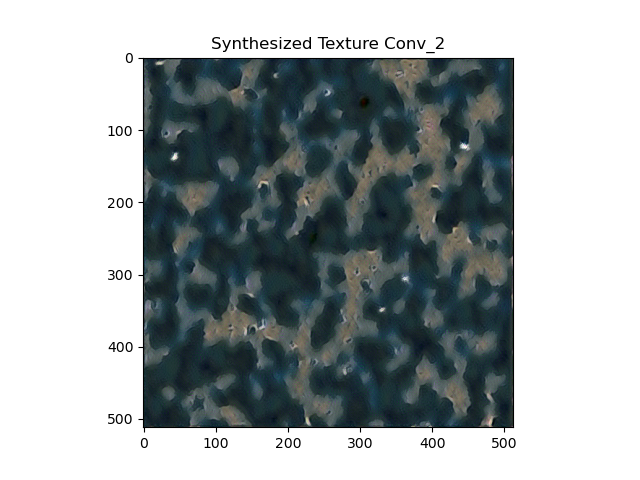
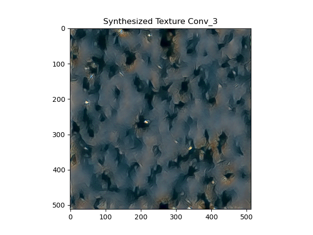
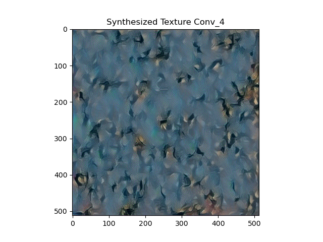
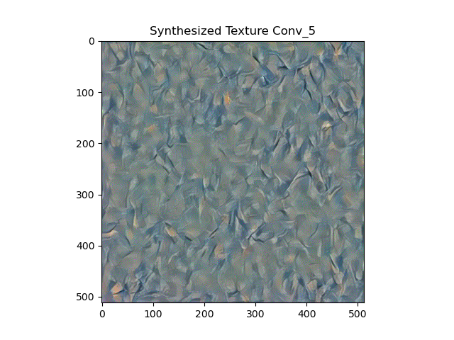
We can see that the first layer has the strongest impact on the style, and the last layer only has few similarity in style with the origianl style image. And the shallow layer has dense and blur style, and the deep layer has light and sharp style. Because we want the style be strong to overwritten the content's original style, the first layer's result is more of what we want. So I focus on the front layer, and incrementally add more layers to the first layer, the results are below:
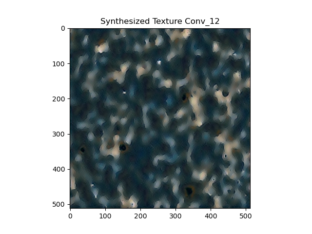
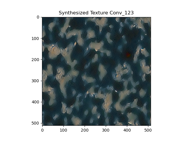
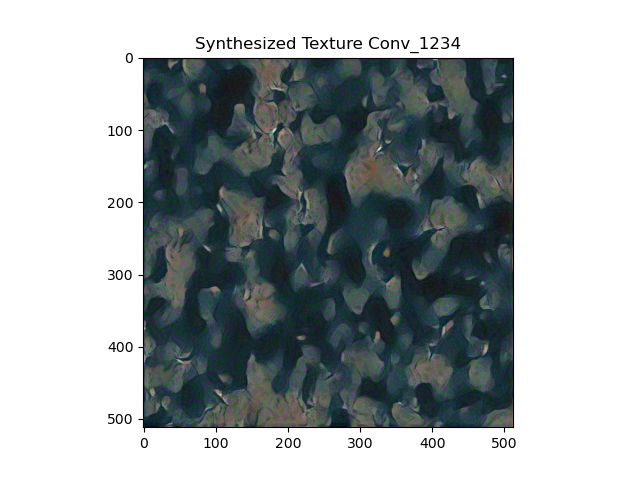
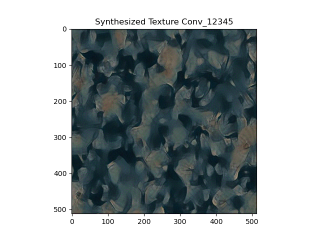
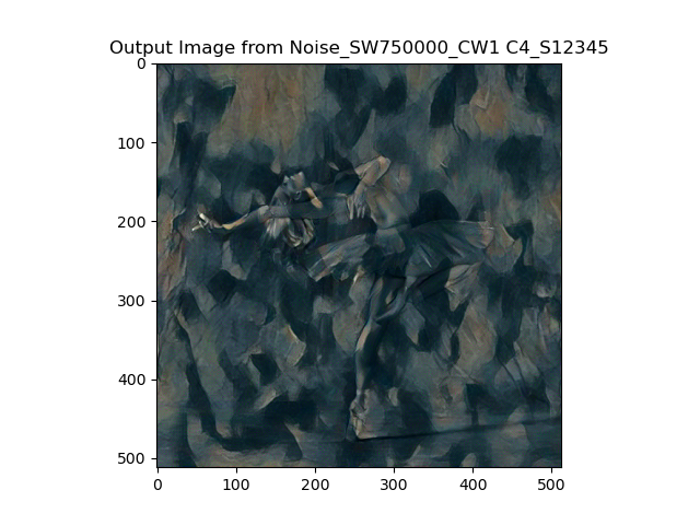
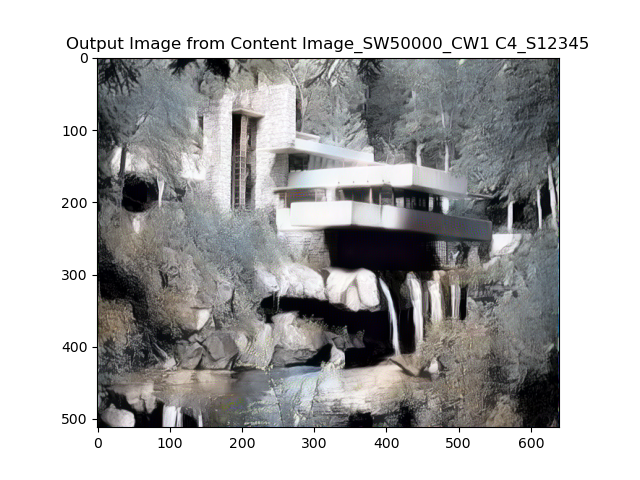
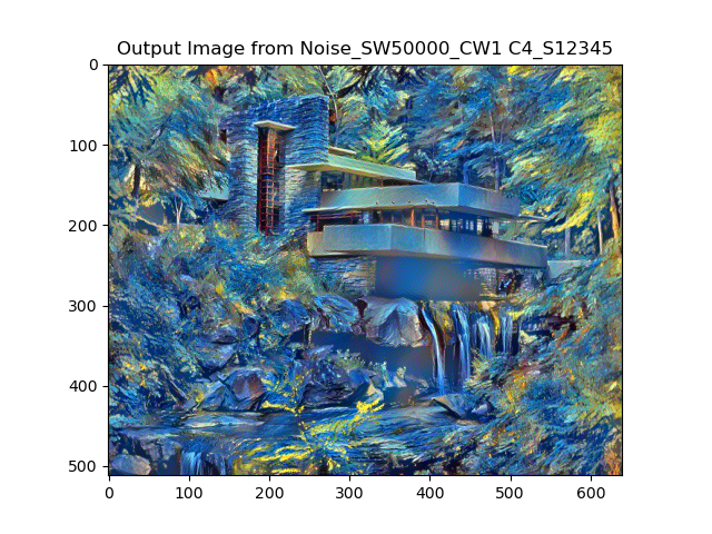
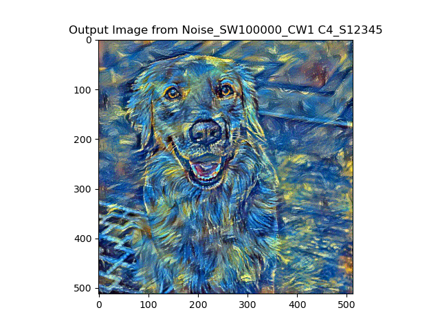
From the results, I have a general feeling that when apply style loss to every layer, the output style image has both good sharpness and densive style, so I choose the layer 12345 for my preference. And I test it with different input random noise, and we can tell that the generated style is visually different just by eye-balled. This means everytime, we can have the similar but different style.
.png)
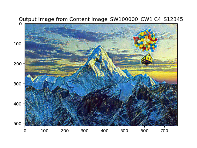
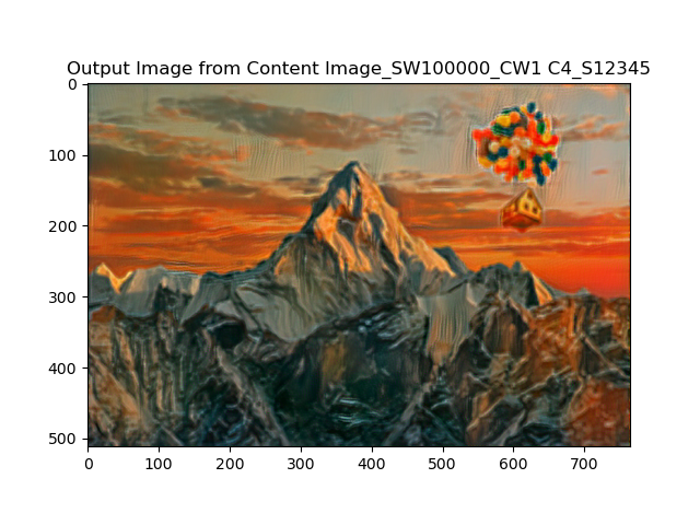
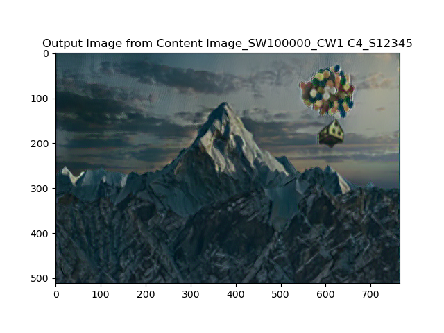
Part 3: Style Transfer
After deciding the content loss and style loss structure, it's time to merge them together in the network. In the implementation, to fit the purpose of merging different size of style and content image, I first resize both of the style and content image's smaller dimension to 512 if using cuda, and because we want to maintain content image as same size and ratio as original input, I fix the content's size, and do first do padding for the case when style image's longer dimension is content image's short dimension, this is because if there is empty(black) part in style image, the style feature can be hugely deprecated. And then I do centerCrop on the style image to fit exactly the same size with content image, this is also because we care more about the pattern and texture of the style image instead of its completeness.
The major hyperParameters are the weights of content and style loss, I fix the content loss weight as 1, and adjust style loss differently, the results are shown below:
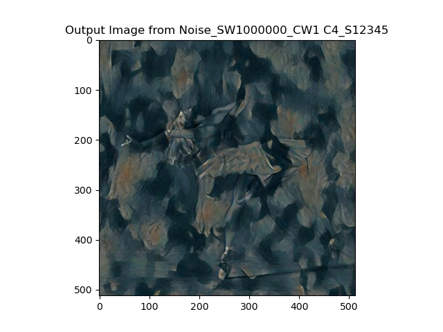
The weight of style loss ranges a big number, as you can see, for weight < 10^4, the style barely works, but when weight> 10^6, it overwrittens the content. Therefore, a good weight is range(10^4,10^6), however, there is no best weight for a general implementaion. I realized the best weight is different for different style and content input. My general choice is around 10^5. For dancing image and picasso style, I choose style weight of 1.5 * 10^5.
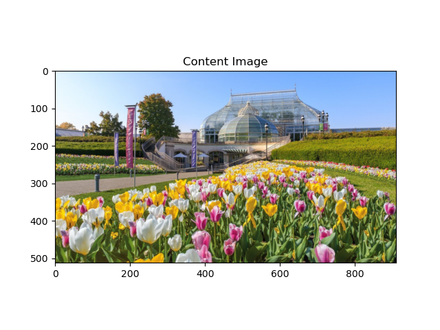
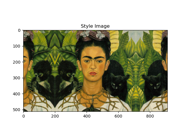
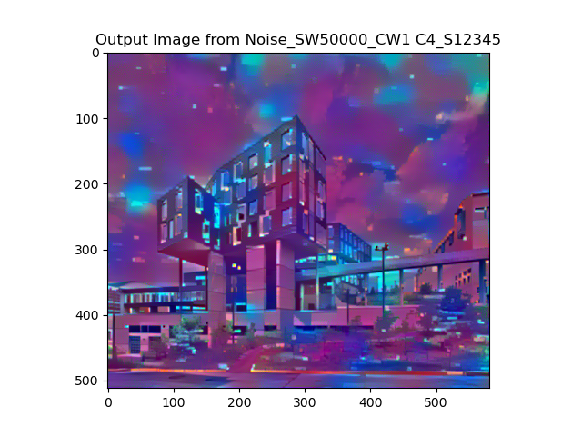
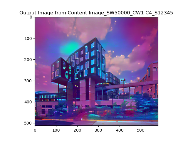
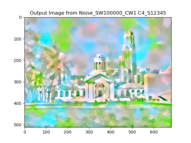
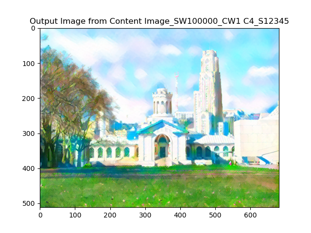
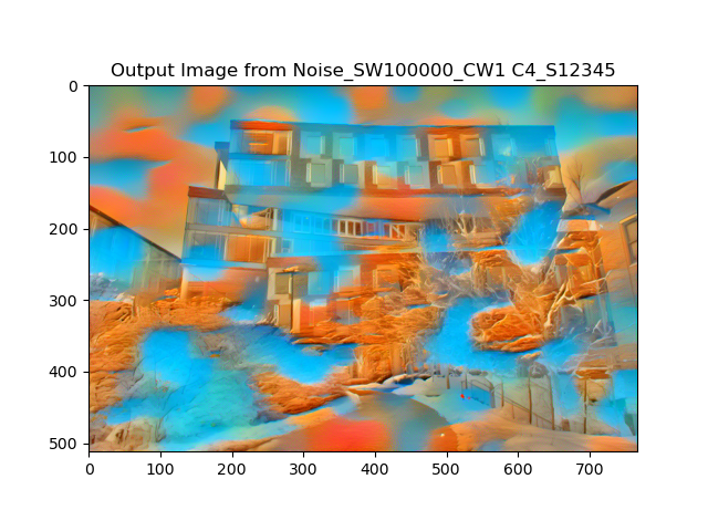
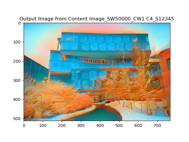
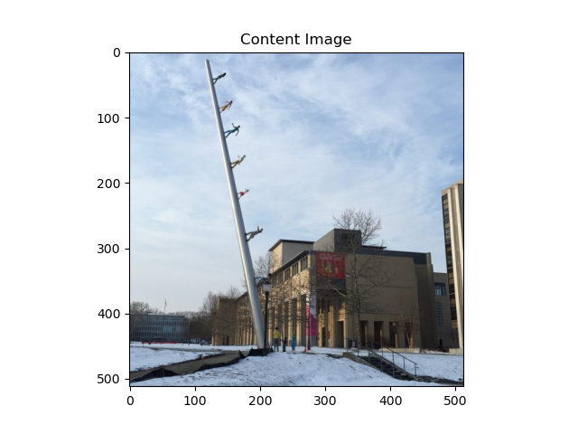
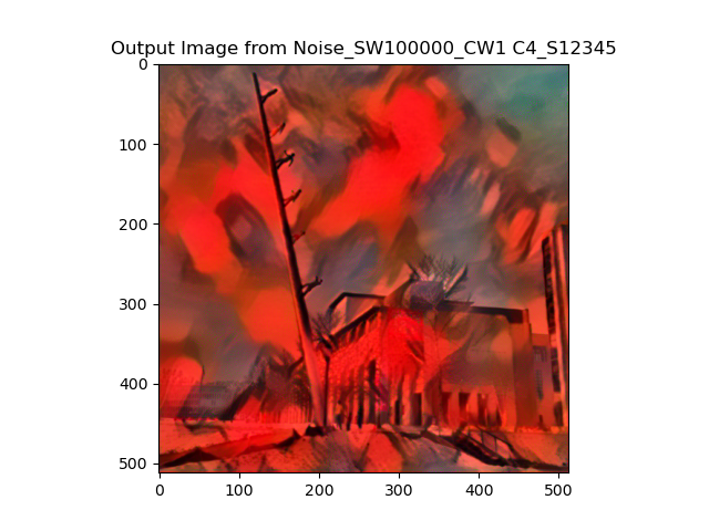
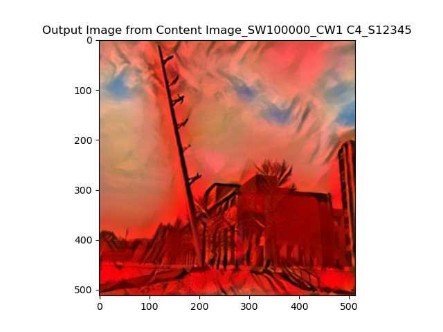
To test the robustness of the implementation, I mix 3 content images and 3 style images to get 9 group of style transfer. The content & style input and the noise-based & content-based output are listed below:
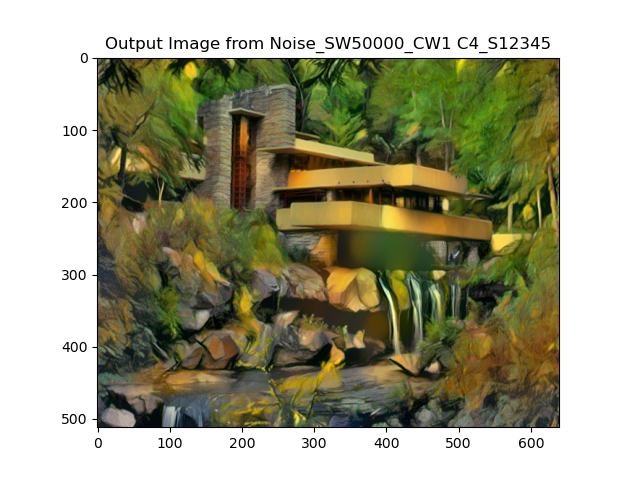
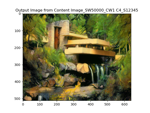
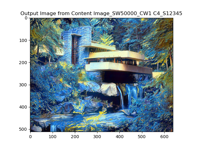
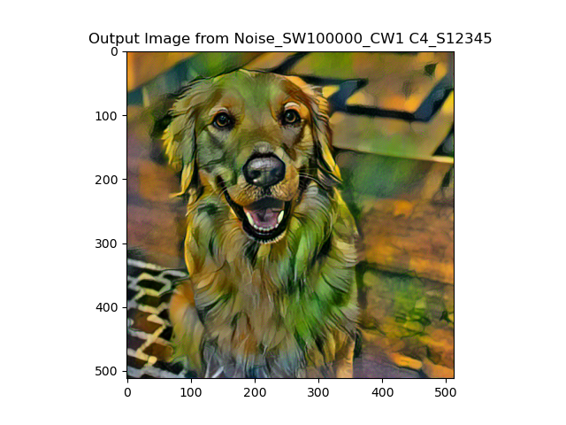
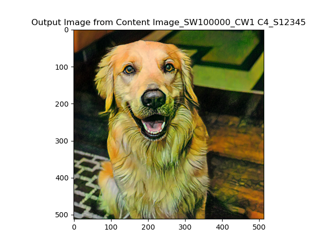
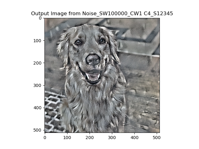
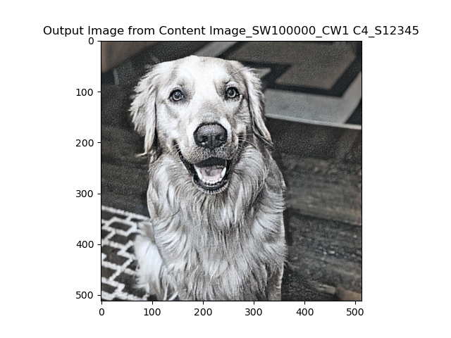
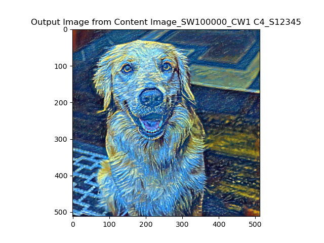
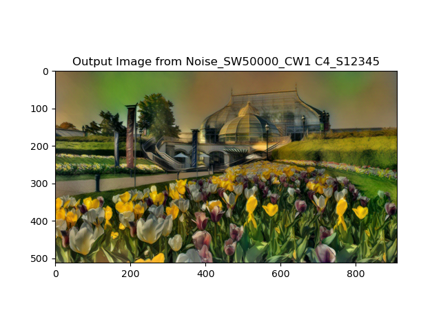
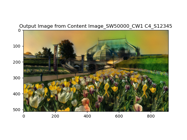
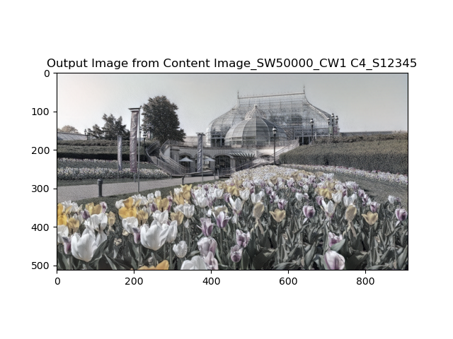
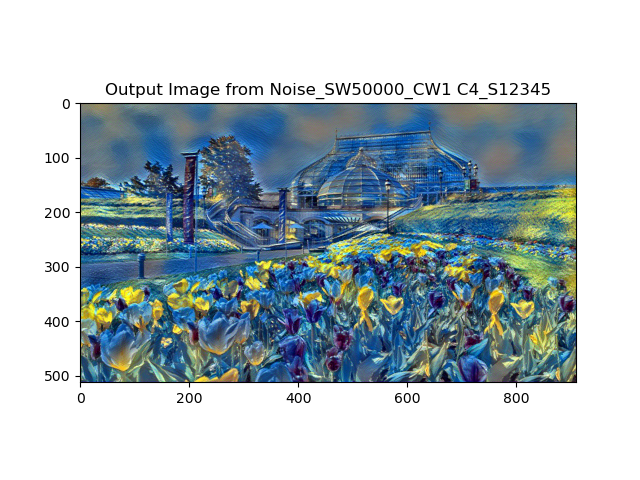
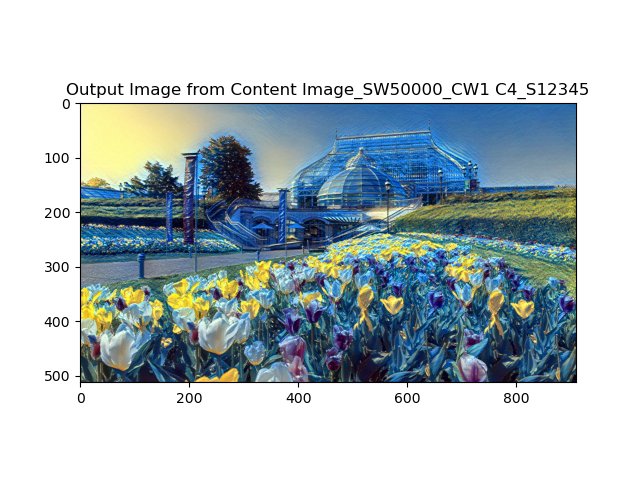
From the experiment, we can tell that images generated from noise and content image are different, and the weight can impact both the output, I export relatively good results for different images combination with different weights. I think the weights depends on the strength of the style image, and the initial color saturation and intensity of content image. By comparison, we can tell that noise generated image has stronger style pattern, and the pattern tends to overwritten the content feature, whereas the content image generated image has good style and content shape at the same time, therefore I mostly use content image to generate outputs for the later section. And the running time varies from image to image, but the average running time goes around 23s for noise image, 19s for content image. It's because the regression loss calculation is more time comsuming for noise task.
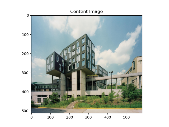
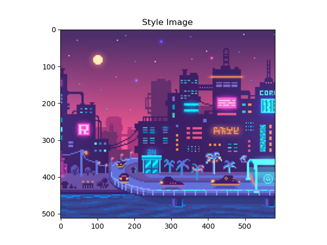
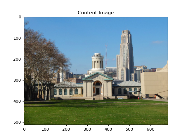
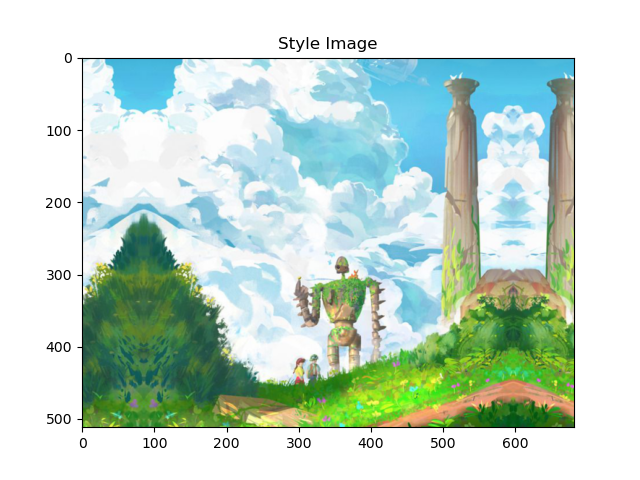
I'm quite interested in the topic of architecture, and I collect a group of CMU campus photos, apply the style transfer on them. Here are the results:
Bells & Whistles
Previous Assignments as Content Image
I choose two outputs from previous assignments of Poisson Blending and CycleGAN, and apply style transfer to them:


Assignment #5
Introduction
In this assignment, we implement a few different techniques to manipulate images on the manifold of natural images. First, we invert a pre-trained generator to find a latent variable that closely reconstructs the given real image. In the second part of the assignment, we take a hand-drawn sketch and generate an image that fits the sketch accordingly.
Part I: Inverting the Generator
For the first part of the assignment, we mainly want to solve an optimization problem to reconstruct the image from a particular latent code. And the loss function consists of two parts: pixel-wise generated image and target(source) image's Lp loss; latent space level of content feature MSE loss. To expand it, we want to optimize the difference between image from StyleGAN2's generator and target image to get the better z input, here I test L1 and L2 loss; and at the same time we want to minimize the distance of manifold content feature between target and the z input, which in our case, we feed them to a VGG-19's feature layers, and get compute the loss of conv_3 and conv_4's output.
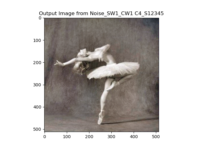
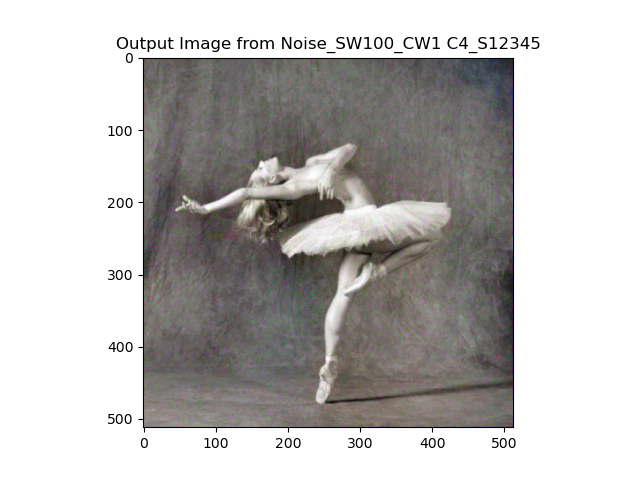
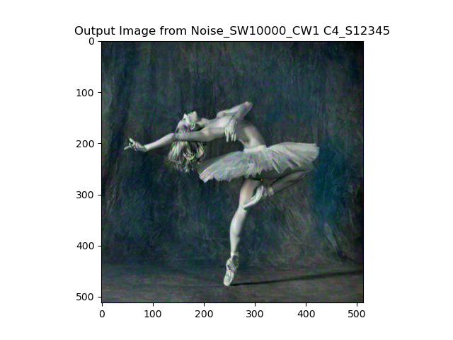
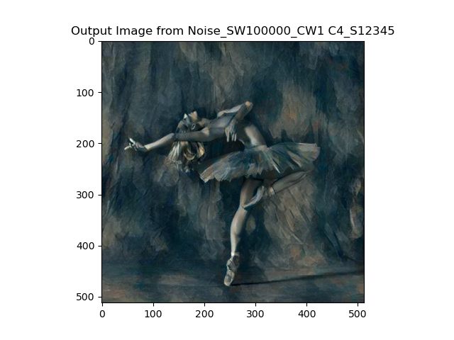
StyleGAN2 has one remarkable feature to mapping Gaussian distribution of z into w or w+ by the mapping layers so that the noise has a better distribution to fit the model. For comparison of different generator, we experiment with both DCGAN and StyleGAN. Also, for noise sampling, we want to test the influence of distribution of the noise, we test with and without mean normalization, for mean we use N=10000 samples. And for the optimization, I use LBFGS. A group of Ablation experiment is listed below:


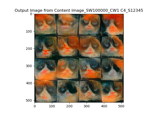
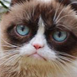
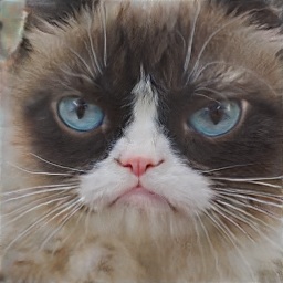
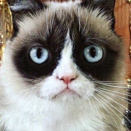
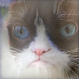
Considering the results above, we decided to use mean w+ samping, stylegan2, l1 norm, l1 weight of 10, perc weight of 0.1 as hyper-parameter to generate the cat. Some of the examples are shown below:


Part II: Interpolate your Cats
For Interpolation, given images \(x_1\) and \(x_2\), compute \(z_1 = G^{-1}(x_1), z_2 = G^{-1}(x_2)\). Then we can combine the latent images for some \(\theta \in (0, 1)\) by \(z’ = \theta z_1 + (1 - \theta) z_2\) and generate it via \(x’ = G(z’)\).
The examples of interpolated gif image are shown below:


Part III: Scribble to Image
We use color scribble constraints in this problem. Given a user color scribble, we would like GAN to fill in the details, it's pretty much similar to the implementation of Part I, except that we want to apply mask of sketch to both target and generated images, and to both their latent variables(here the mask use pooling to downsize to the same size of latent dimension). The results are shown below:


Bells & Whistles (Extra Points)
High Resolution Cat Dataset
We used the dataset from 256/128 Resolution Cat Dataset, and generated images like below:
AdaWild Dataset
Also, I tried AdaWild Dataset and got results as below: