Joshua Cao | Carnegie Mellon University
About Course
16-726 Learning-Based Image Synthesis / Spring 2022 is led by Professor Jun-yan Zhu, and assisted by TAs Sheng-Yu Wang and Zhi-Qiu Lin.
This course introduces machine learning methods for image and video synthesis. The objectives of synthesis research vary from modeling statistical distributions of visual data, through realistic picture-perfect recreations of the world in graphics, and all the way to providing interactive tools for artistic expression. Key machine learning algorithms will be presented, ranging from classical learning methods (e.g., nearest neighbor, PCA, Markov Random Fields) to deep learning models (e.g., ConvNets, deep generative models, such as GANs and VAEs). We will also introduce image and video forensics methods for detecting synthetic content. In this class, students will learn to build practical applications and create new visual effects using their own photos and videos.
Assigment Summary
| Topic | Abstract | Reference | |
|---|---|---|---|
| A1 | Colorizing the Prokudin-Gorskii Photo Collection | Implement SSD, pyramid structure, USM, auto crop, contrast methods |
Dataset USM Hough Transform |
| A2 | Gradient Domain Fusion | ||
| A3 | When Cats meet GANs | ||
| A4 | Neural Style Transfer | ||
| A5 | GAN Photo Editing |
Copyright
 All datasets, teaching resources and training networks on this page are copyright by Carnegie Mellon University and published under the Creative Commons Attribution-NonCommercial-ShareAlike 4.0 International License. This means that you must attribute the work in the manner specified by the authors, you may not use this work for commercial purposes and if you alter, transform, or build upon this work, you may distribute the resulting work only under the same license.
Assignment #1
Introduction
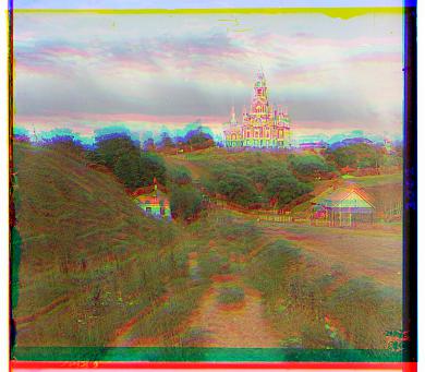
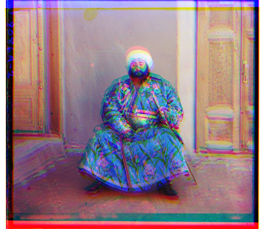
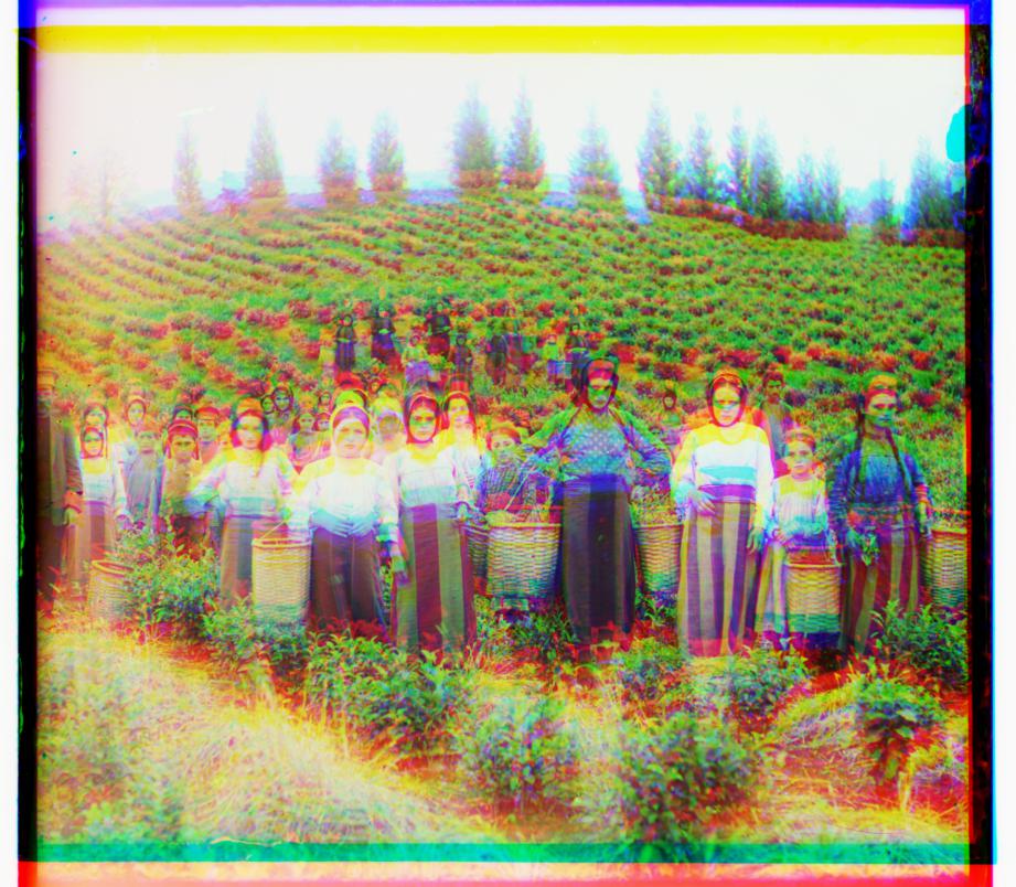
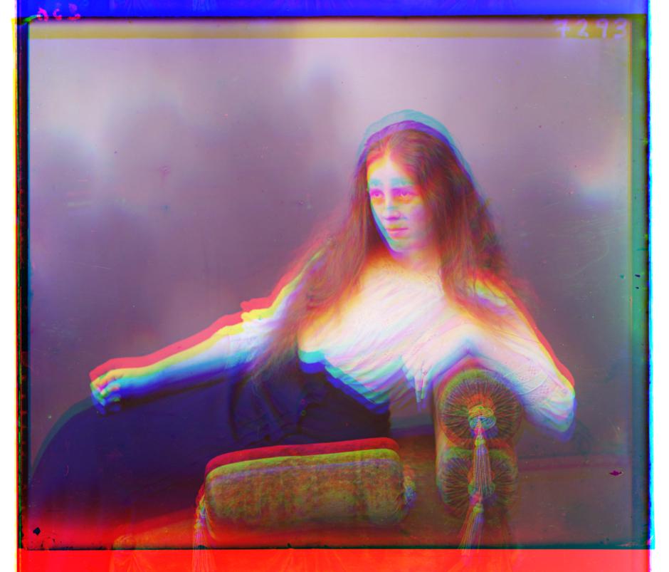
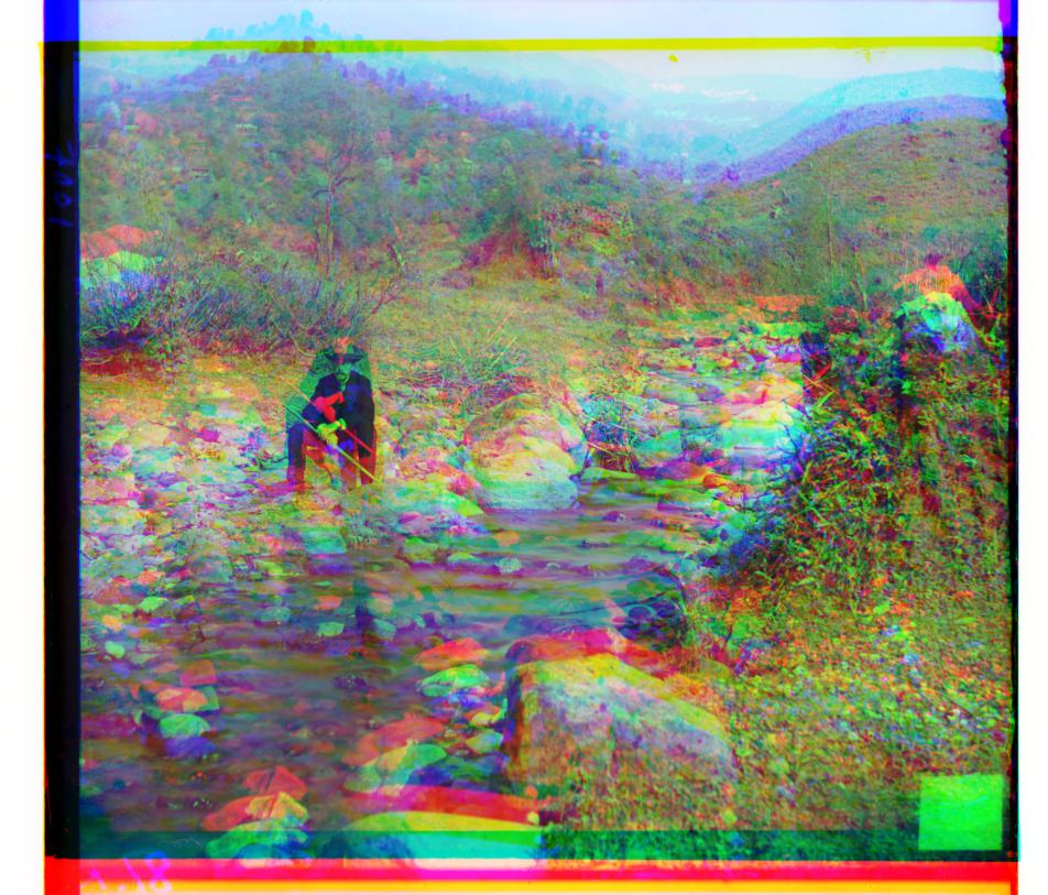
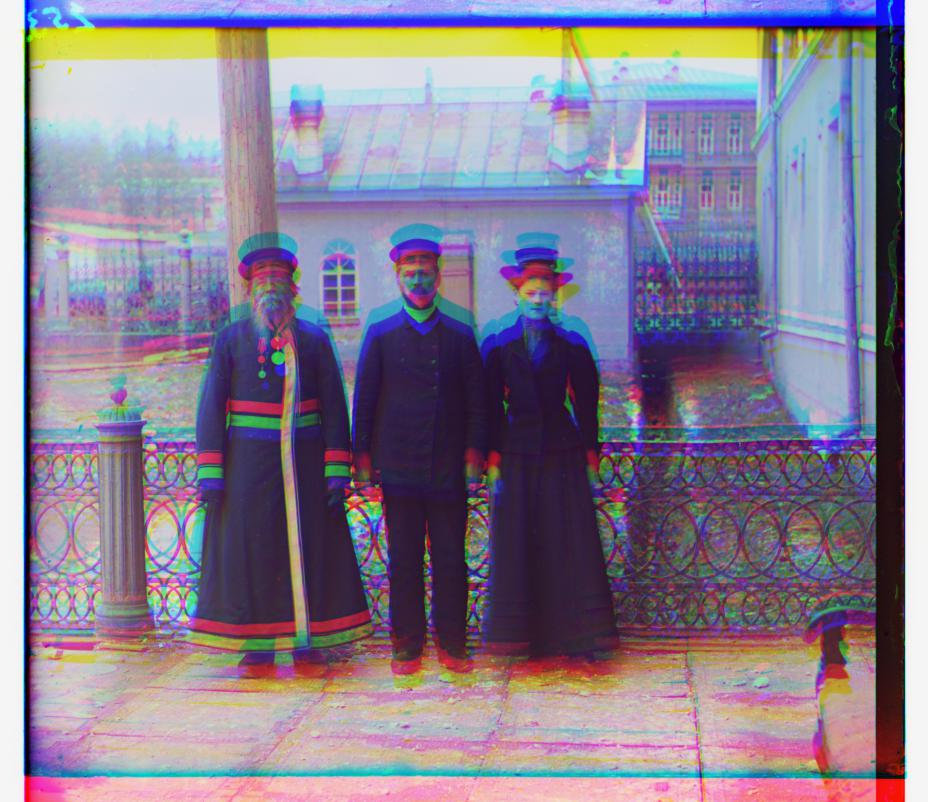
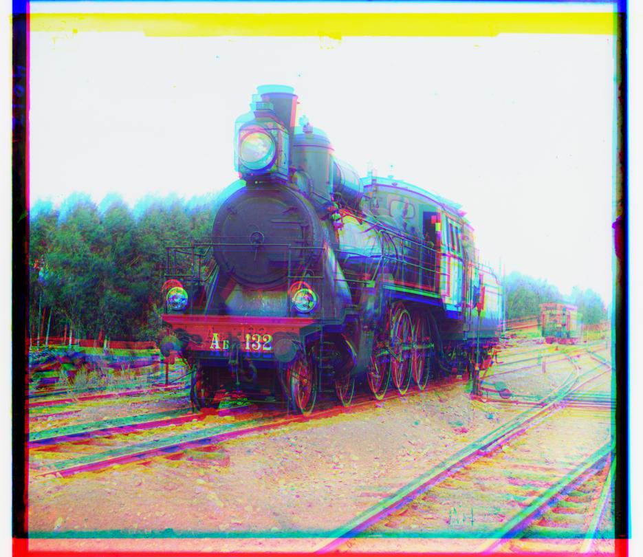
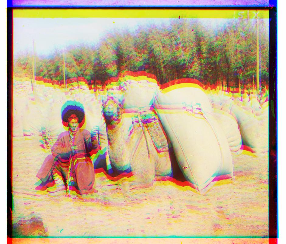
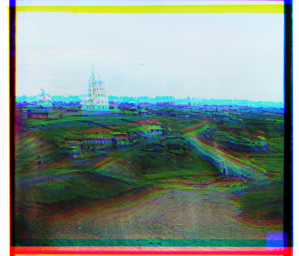
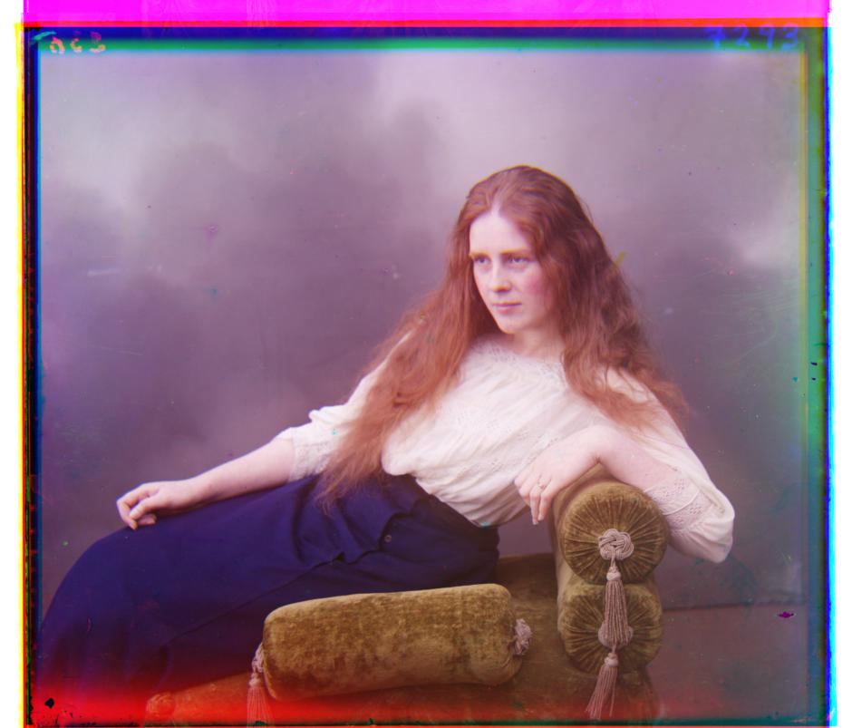
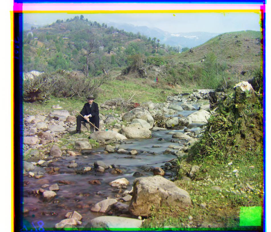
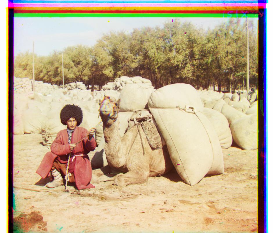
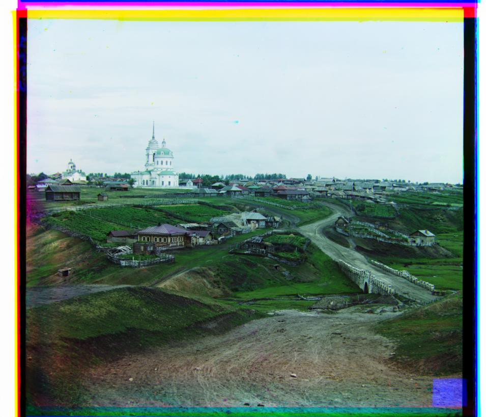
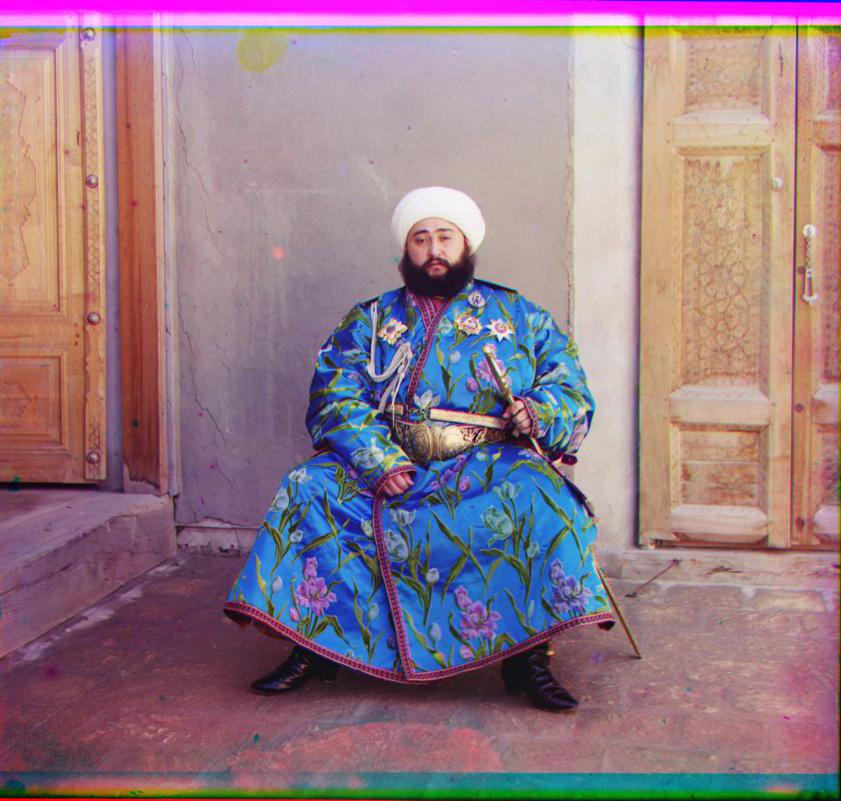
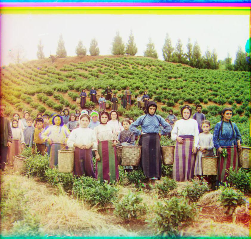
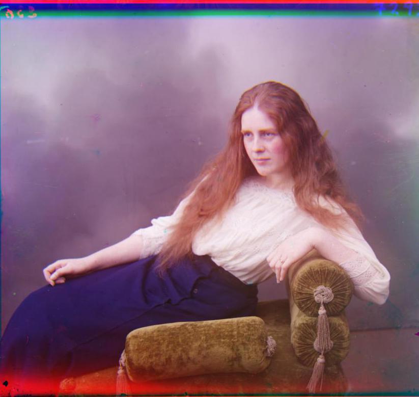
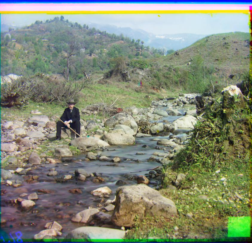
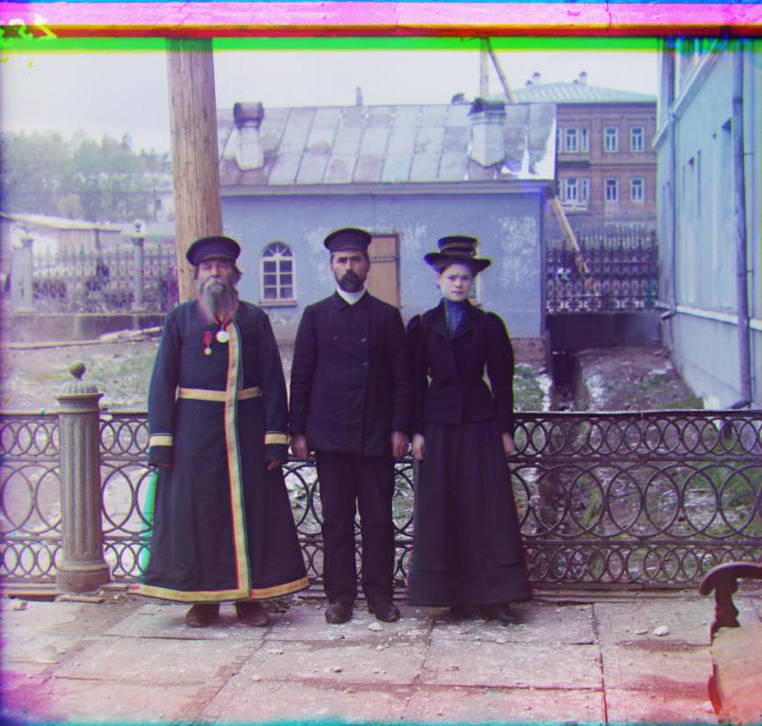
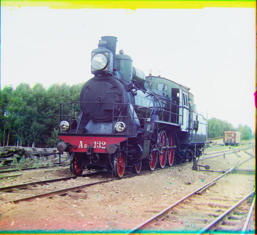
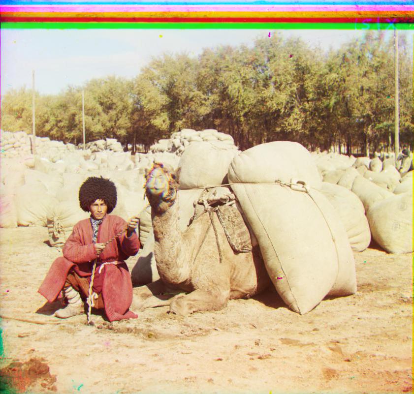
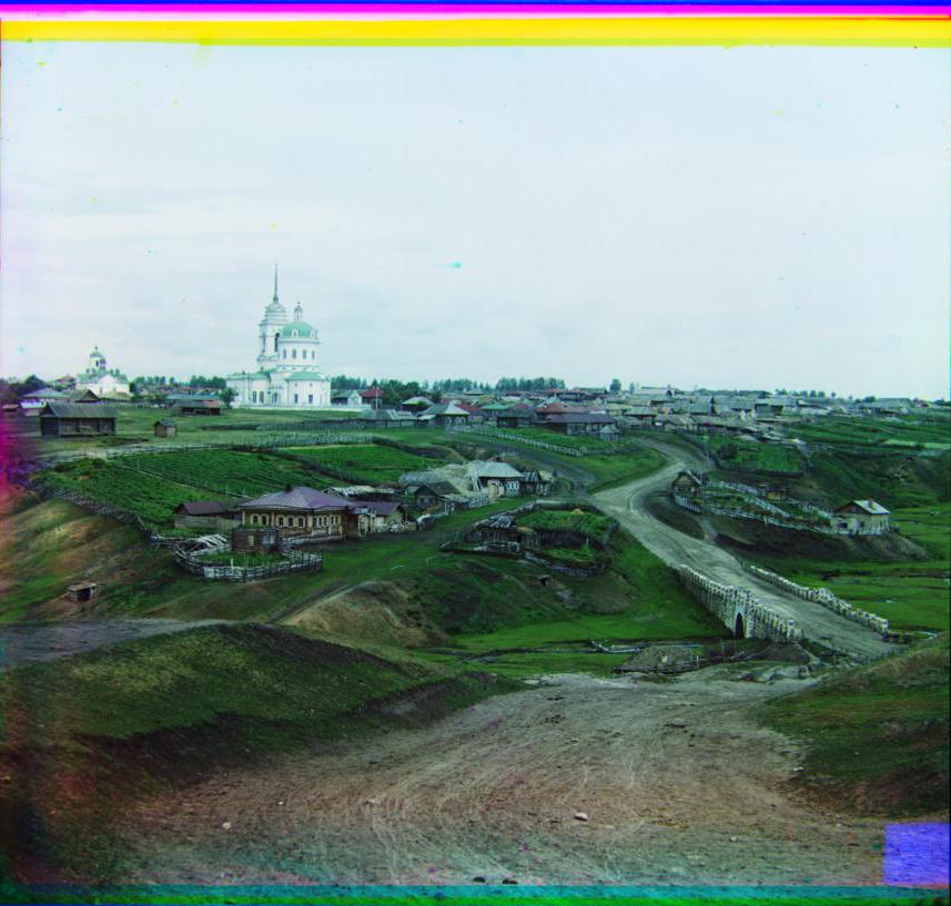
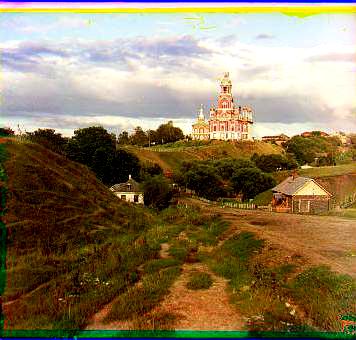
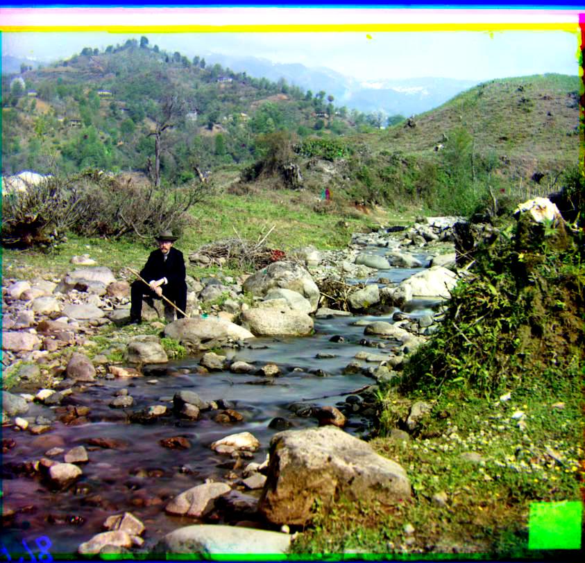
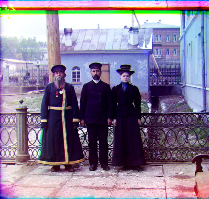
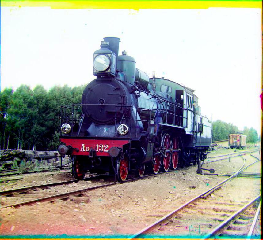
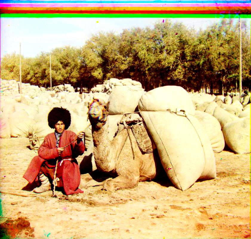
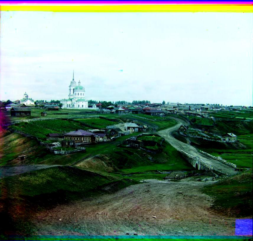
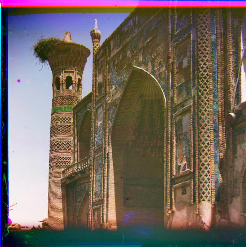
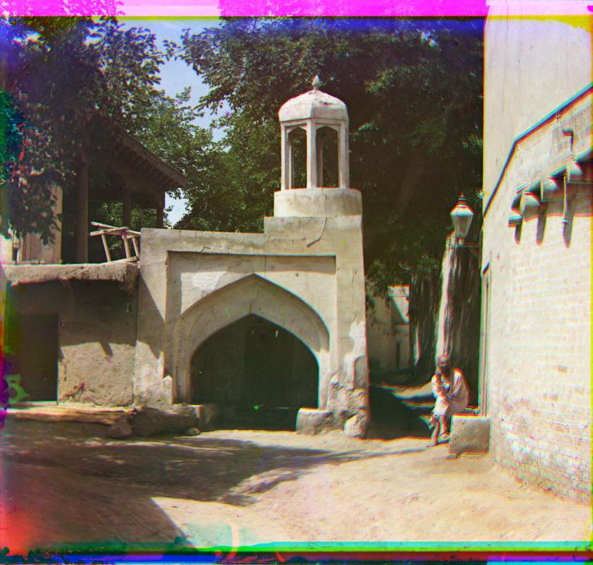
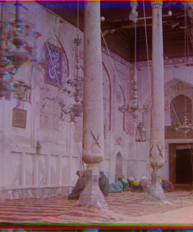
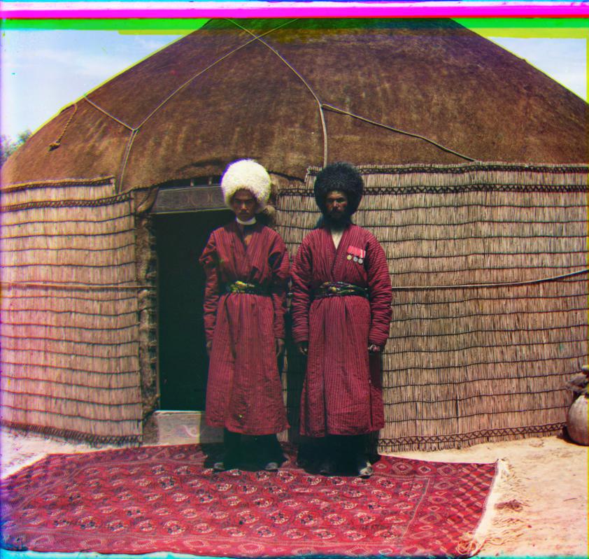
The Prokudin-Gorskii image collection from the Library of Congress is a series of glass plate negative photographs taken by Sergei Mikhailovich Prokudin-Gorskii. To view these photographs in color digitally, one must overlay the three images and display them in their respective RGB channels. However, due to the technology used to take these images, the three photos are not perfectly aligned. The goal of this project is to automatically align, clean up, and display a single color photograph from a glass plate negative.
Direct Method
Before diving into algorithms, I decide to blend R, G, B images directly and have an intuitive feeling of the tasks, which at the same time provides a reference to compare how far my algorithm can go. There are total 1 small jpeg and 9 large tiff images from the given dataset. Their direct blending goes as below:
SSD & NCC Alignment
I implement both SSD and NCC to compare the small patch's similarity for alignment, the search range is [-15,15], and the algorithm works both well on the small jpeg image as shown below. To speed up the calculation, I also cropped 20% of each side of the image to decrease calculation on the edge. However, to deal with larger image, not only the search range is not large enough, but also the calulation takes extremely long. Therefore, the pyramid structure comes to practice.
Pyramid Aligment
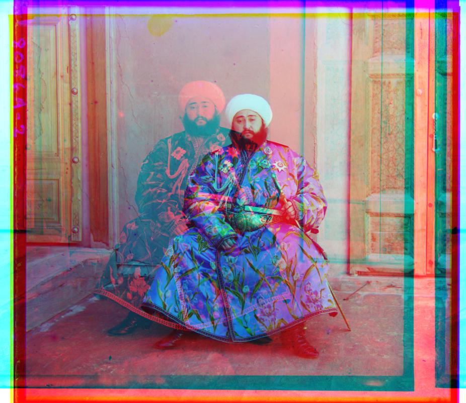
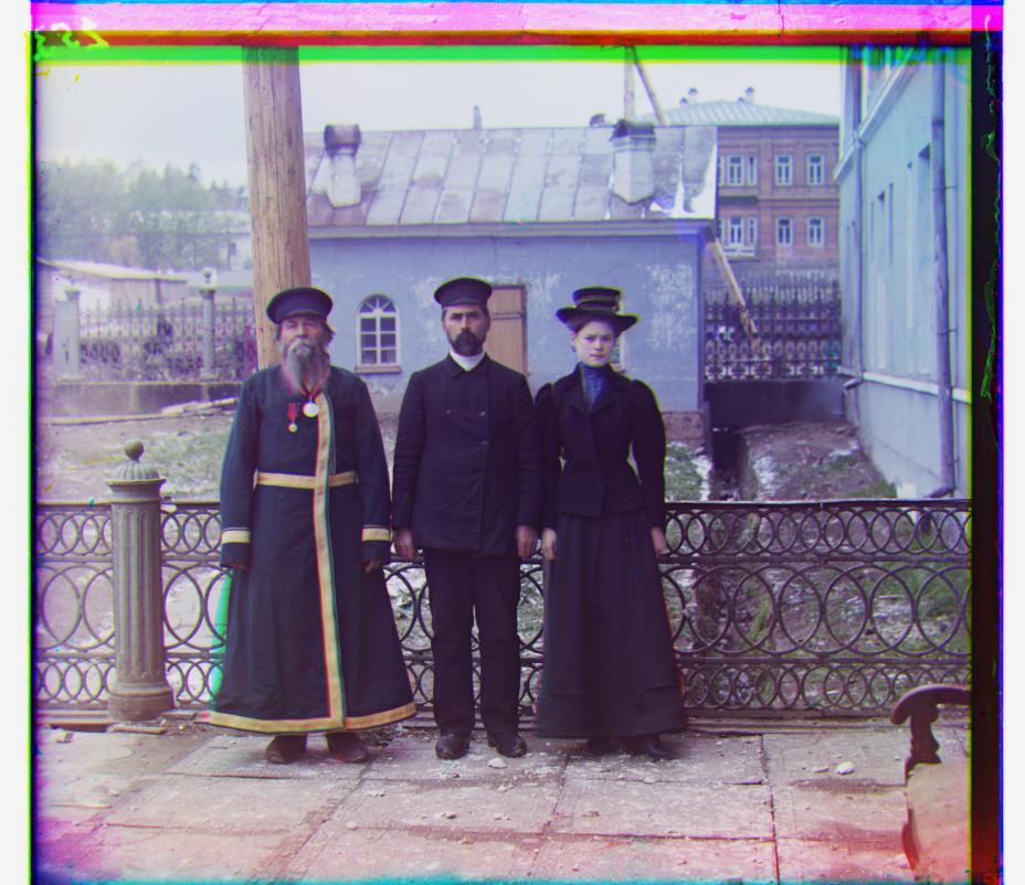
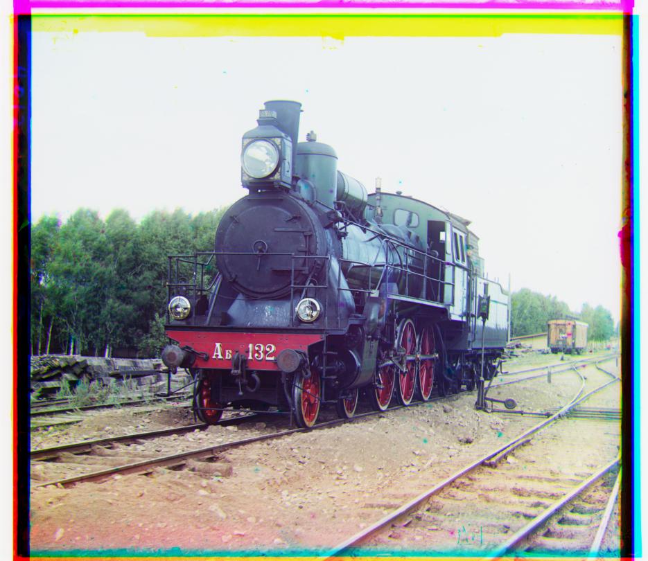
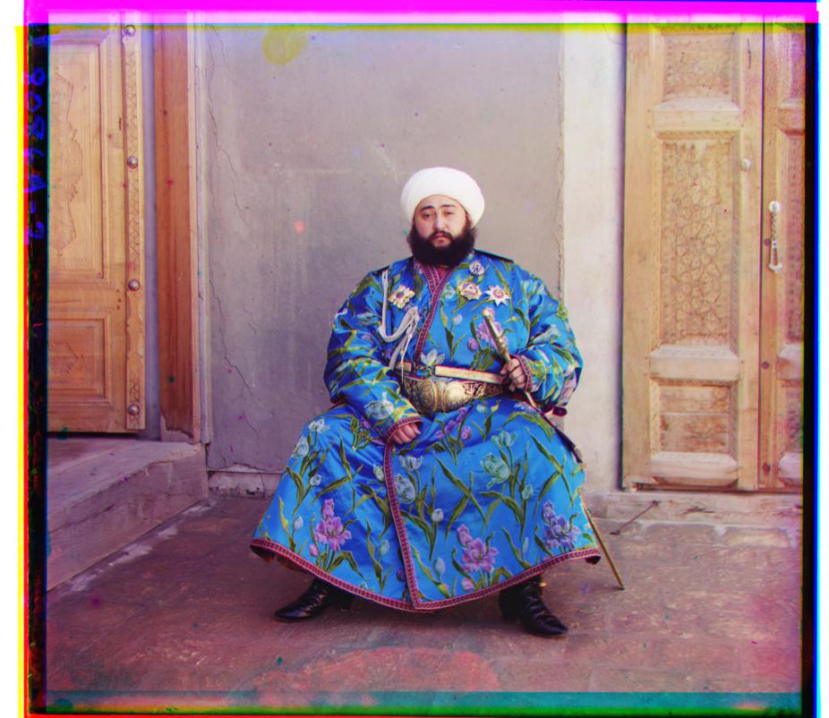
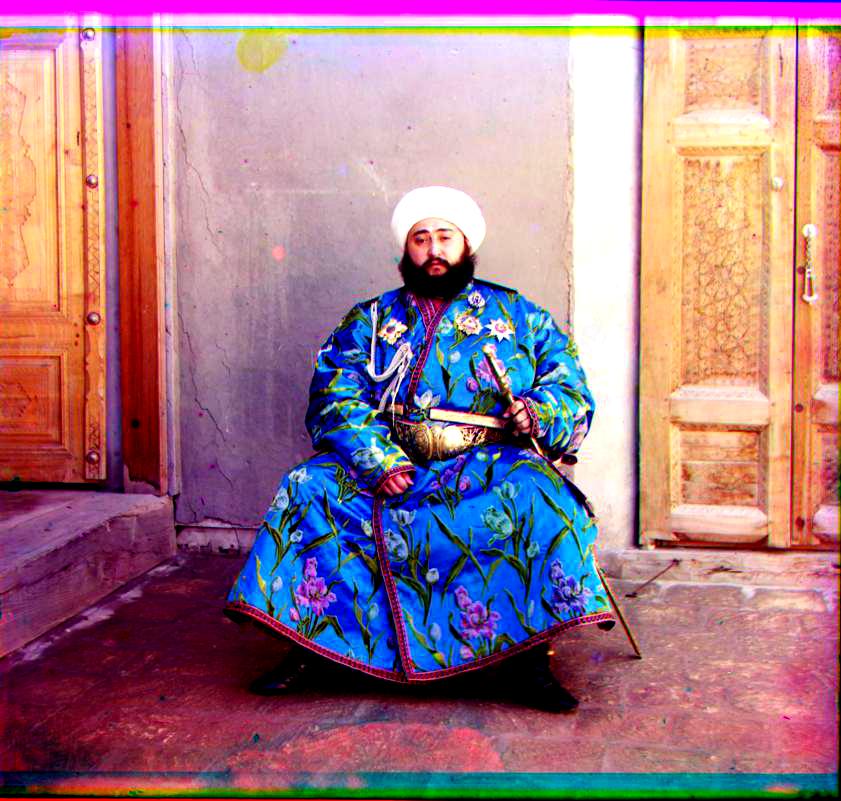
I use log2(min(image.shape)) to find out how many mamixmum layers the image can have, and add conditions to only apply the pyramid algorithm for images larger than 512*512, and the small image can directly use [-15,15] SSD search. For large images, my starting layer is a size around 265 pixels(2^8 as first layer), and exhaustively search till the original image size, because I realized missing final layer will give me color bias all the time(misalignment of color channel is very easy to detect even though it's just small pixels). The first implementation of my method took 180s for one image. To speed it up, I recursively decrease search region by 2 each time to shorten it to 55 seconds per iamge, because the center of search box is determined by last layer, so the deeper algorithm search, the smaller search range it requires to find the best alignment. The output is listed as below. As you can see, most of the images are aligned quite well but image like the piece of Sergei Mikhailovich Prokudin-Gorskii, work even worse than direct alignment, this is because the brightness of the images are different, therefore, I use an USM(Unsharp Mask) algorithm to fix the issue.
Extra Credits
USM Unsharp Mask
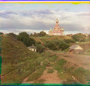
The USM algorithm is mainly to sharpen or soften the edge of images, and allows accurate SSD difference to make better alignment. The algorithm is called for each recursion in the pyramid alignment, and it first uses Gaussian Blur to blur the single channel(gray) image, and subtract it from the original image, then I take the region of difference that is larger than certain threshold and subtract them from the original image and multiple certain constant parameters. Here I use subraction because I notice certain edge needs to be softened instead of being sharpened, due to some disturbing edges stand out too much in the original image that makes SSD find the wrong alignment. The USM specifically improves the quality of this image:
Crop Image
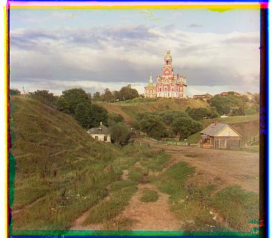
To get rid of the borders, I mainly use two cropping method, the first one is to keep area only for all three channels have contents, and remove those blank area caused by alignment, this is implemented by retriving shift of each single channel image. But this method can't deal so well with the region that is originally black or white outside the image. Then I use a MSE(Mean Square Error) method to calculate each row and each column's error, and set up when three adjacent rows or columns all are smaller than certain threshold, it is the area should be cropped. The result shows as below:
Add Contrast
The contrast method is pretty straight-forward, I just calculate the accumulative histogram of the image, and take 5% and 95% as 0 and 255 respectively, and stretch the color value in between so that the contrast of the main image increase.
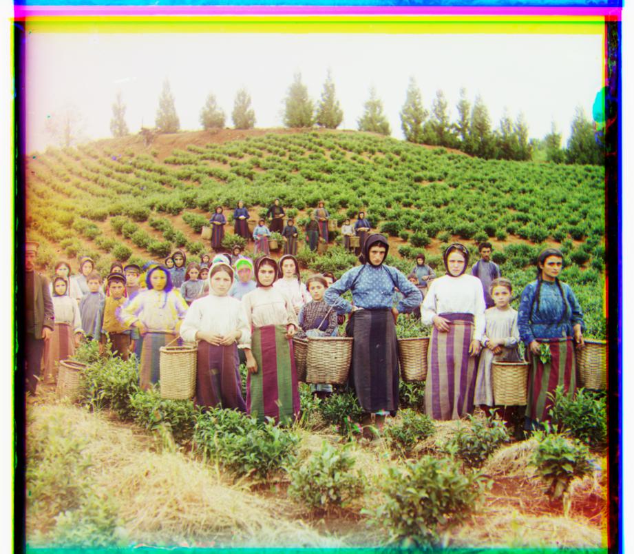
Other Dataset
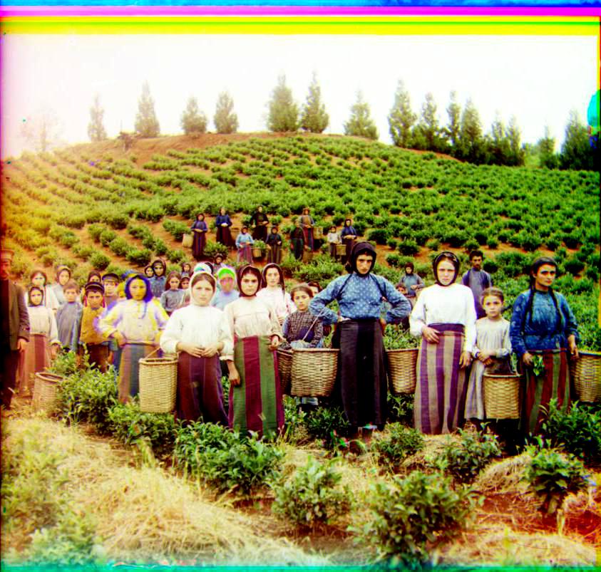
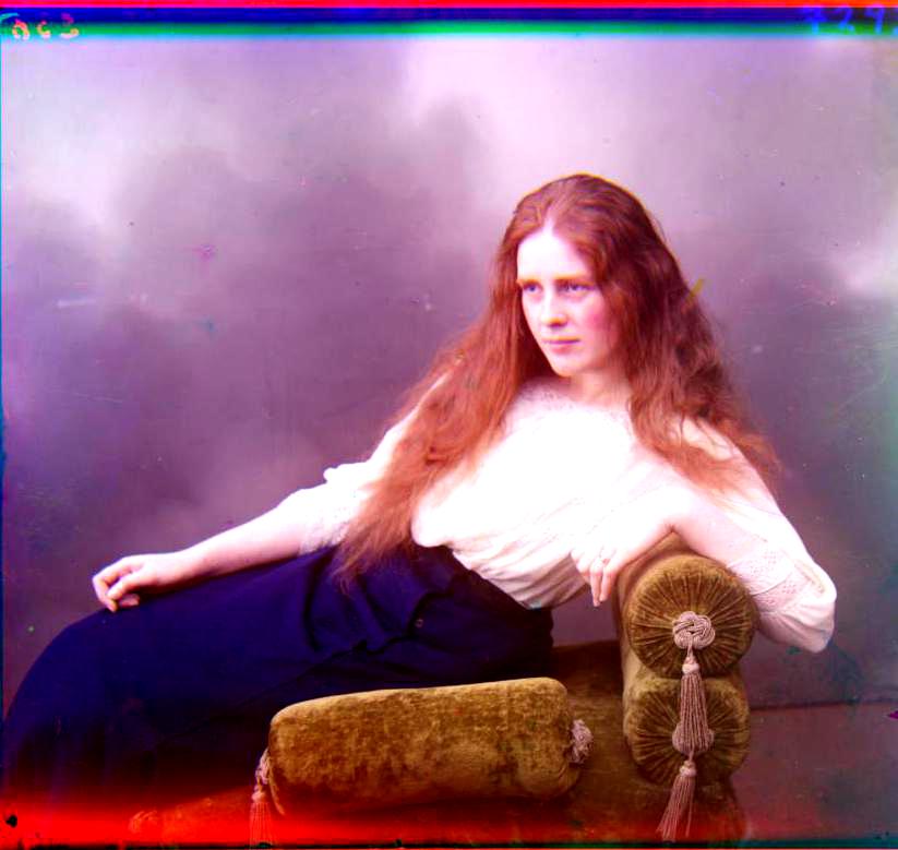
I find some other similar dataset that has pretty large tiff image to test the algorithm. The result shows as below
Assignment #2
Introduction
The project explores the gradient-domain processing in the practice of image blending, tone mapping and non-photorealistic rendering. The method mainly focuses on the Poisson Blending algorithm. The tasks include primary gradient minimization, 4 neighbours based Poisson blending, mixed gradient Poisson blending and grayscale intensity preserved color2gray method. The whole project is implemented in Python.
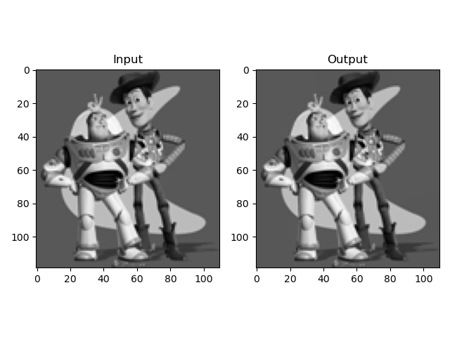
Toy Problem
The toy problem is a simplifed version of Poisson blending algorithm, therefore it helps understanding the Poisson blending a lot. The major functions are three, to calculate the gradient of x axis and y axis, and to align the left-top corner (0,0) of the image:
((v(x+1,y)−v(x,y))−(s(x+1,y)−s(x,y)))**2
((v(x,y+1)−v(x,y))−(s(x,y+1)−s(x,y)))**2
(v(1,1)−s(1,1))**2
We use the equations to loop through each pixel of the source image to construct A and b. By solving the least square form of Av=b, we can get the synthesized image v. Say the given gray image size is H by W, A's dimension is H*W by 2*H*W+1, b's dimension is H*W by 1. The result is pretty much to test if we can copy the original image, as shown below:
I implemented it in both loop method and non-loop method, the interesting thing is that with loop method, it only takes around 0.4s, whereas with the non-loop method, which is supposed to be faster in Python environment than loop, turns out to take around 10s. I think the major reason is that sparse matrix's arithmetic calculation is more expensive than directly assign value to coordinates. In the non-loop method, I mainly use lil_matrix to construct sparse matrix, and use np.roll, np.transpose to construct A matrix. Finally I decide to use the loop method for the rest of the task.
Poisson Blending
Based on toy problem's hint, Poisson Blending explores the four neighbour of each pixel, follow the equation below that v is the synthesized vector that we need to solve, s is the source image in the size of target image(but we're only interested in the masked source image), t is the target image:
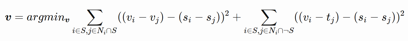
In the equation, each i deals with 4 j, i.e. the same i is calculated 4 times with 4 different neighbour j. The left part considers the condition if all the neighbour of i is still inside the mask, and the right part considers the neighbour not all inside the mask. Notice the difference in code is that for the right part, tj is used to construct parameter b, whereas for the left part, vj is used to construct parameter A.
Also, the given image now has RGB, 3 channels, therefore we need to calculate each channel separately. When I implemented it, I consider that A matrix is always the same for 3 channels, but b are different for each channel, therefore I only calculate A once and b 3 times to speed up the algorithm. What's more, since the we only need to generate image from the maksed source image's coordinate, I only loop through this area to speed up. And finally I merged three v together to get new RGB image. The average speed is related to the image size, to deal with the given example of 130x107(source image) and 250x333(taget image), it generally takes around 20s.
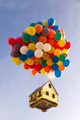
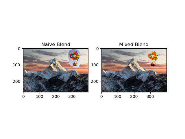
However, the naive Poisson Blending has some issue to deal with blending the image seamlessly, which is because only considering the source neighbour is not enough for strong difference of target and source images. As you can see the image below, the inner part of the ballon house is little blur and not blended so well with the background. Therefore, we need to implement Mixed Blending.


Extra Credits
Mixed Gradients
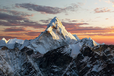
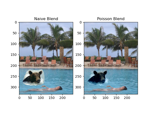
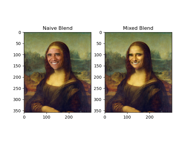
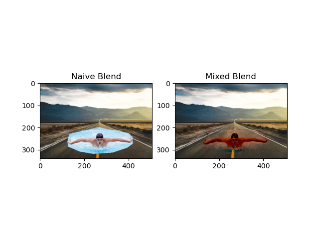
Mixed gradients is actually pretty straight forward based on Poisson Blending, we just add one condition that instead calculating the gradient of source image s, we compare the gradient of s and gradient of t, and take the larger one so that it can better blend when the difference of source and target image are large. The comparison of the same image can be seen as below(The left is blendered without Mixed gradients.):
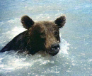
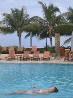
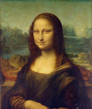
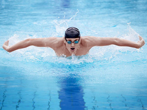
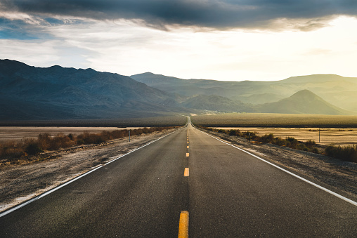
The given example of bear and pool is below:
There are some more generated blending images:
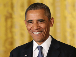
And there is a failure case where the colorful Patrix can't blend so well with the gray-scale like moon image:
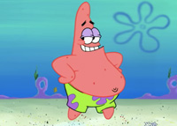

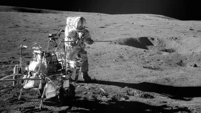
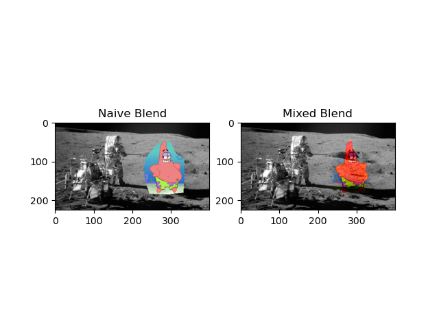
This is mainly because there is upper limitation of the blending algorithm to adjust the color, if the source image and target image have too large difference, the algorithm will reach its limitation to find the solution that best approximate the least square function.
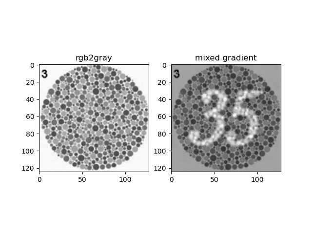
Color2Gray
The Color2Gray method first turns RGB image to the HSV color space, and only consider the S and V channels to represent the color contrast and intensity respectively. In this way, we can keep the color contrast of rgb image and preserve the grayscale intensity at the same time. The algorithm runs similar to the Mixed Gradient where source and target image are S and V. The result is shown as below:
Assignment #3
Introduction
This project implements two famous GAN architecture: DCGAN and CycleGAN. It is programmed in Pytorch, the major code includes the build-up of discriminator and generator neural network, loss function, forward and backward propagations. It also explores different methods that help GAN generate better results, such as Data Agumentation, Differentiable Augmentation, variance of different lose functions, variance of different discriminators, and implemented in different dataset to check the robustness fo the network.
Part I: Deep Convulotional GAN
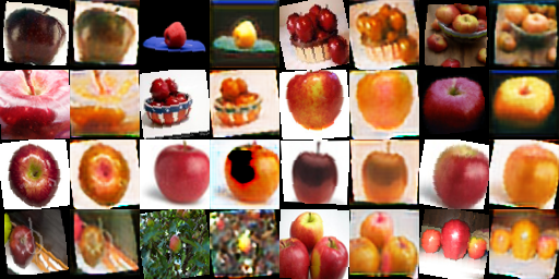
Implement Data Augmentation
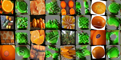
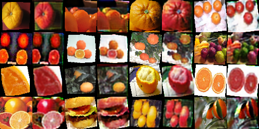
In Pytorch, data augmentation is invoked each time when iterated through the mini-batch, the purpose of the data augmentation is add variance to the dataset, which is especially useful when the dataset is small or each sample of the data are too similar. For example, in this DCGAN training, we only have 204 images as dataset. I mainly use the Resize + RandomCrop, RandomHorizontalFlip, RandomRotation(10 angles) to generate augmentation. The example of orignal dataset and augmented dataset, and GAN generated sample by different dataset can be see here:

The Discriminator
The discriminator in this DCGAN is a convolutional neural network with the following architecture:
According to the formula (N-F+2P)/S + 1 = M(We don't consider dilation here), where N is the input number of channels, M is the output number of channels, S is stride, P is padding, F is size of filter/kernel, since we want N=2M, and we use filter size of 4, stride of 2, we can calculate that padding P is 1. Besides, I use softmax for the output layer, and later on squared mean difference for loss function, since this Discriminator is a classification problem, the softmax-loss combination is a generally good choice.
The Generator
The generator in this DCGAN is a convolutional neural network with the following architecture:
In the generator neural network, I use transposed convolution with a filter, size of 4, stride of 1 and padding of 0 for the very first layer that from 100x1x1 input to 256x4x4 output. And the rest layer all are upsampling of 2, with a filter, size of 3, stride of 1 and padding of 1 to satisfy the condition that output dimension is the 2 times of input dimension. And the reason why the first layer is a transposed convolution is that it has better performance than direct upsampling for noise.
The Training Loop
The training loop including loss function and backpropagation is as straight forward as image below:
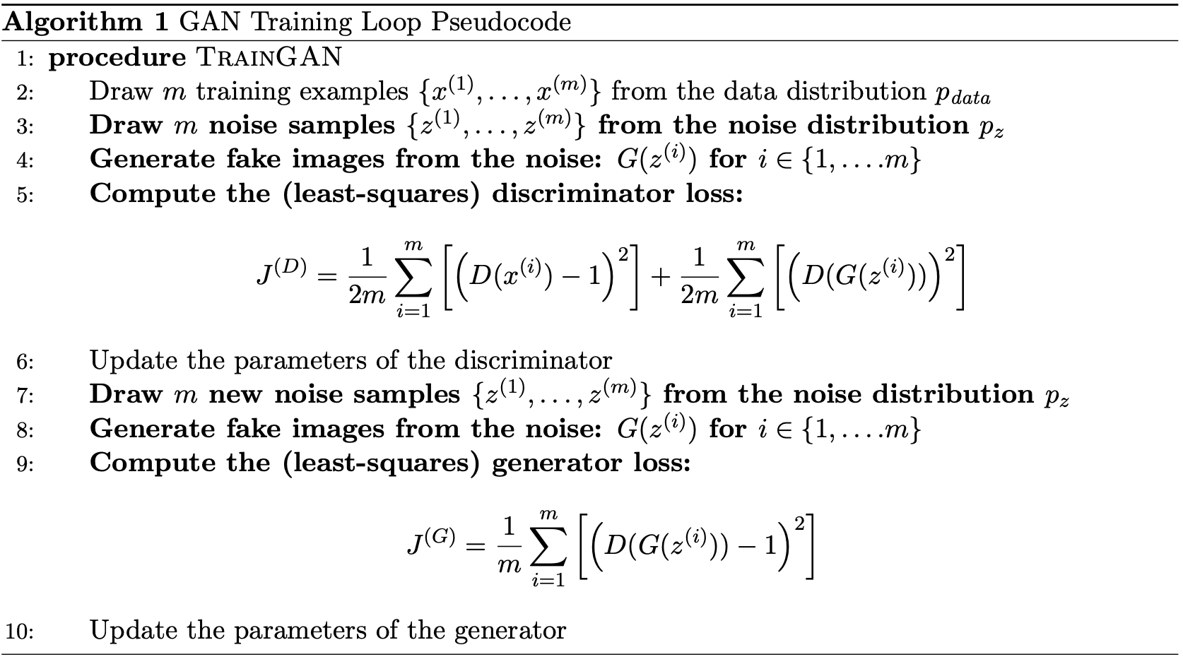
One thing to notice is that we normally first do the back propagation to update the gradients and weights of discriminator, then do the generator, this is because the loss function first goes back to discriminator then to the generator. To better train generator's weight, we prefer the gradient and weights of discriminator is static than dynamic.
Similarly, when training the discriminator, we don't want to update the gradient all the way back to generator, therefore we have to set no_grad_up for the fake_image that is generated from generator and fed to discriminator. In my case, I use torch.detach() function.
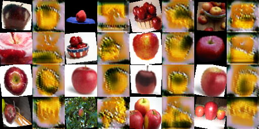
The Differentiable Augmentation
The Differentiable Augmentation method is meant to process data during the training process, it can slow down the training but can significantly improve the output's performance. And it's shown as below:
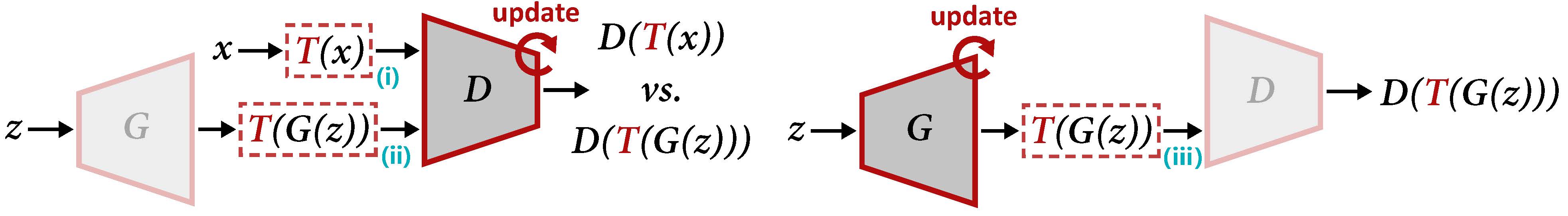
I apply differentiable augmentation to all the generator generated fake images and real images during the training process.
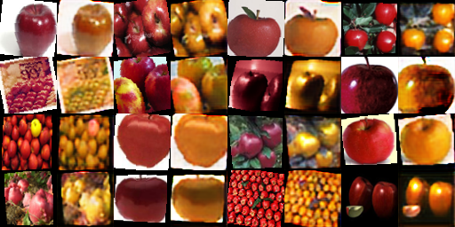
Results
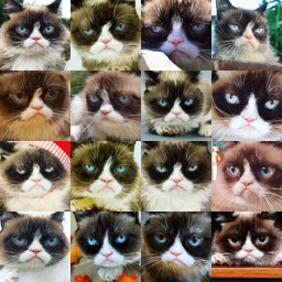
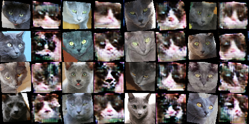
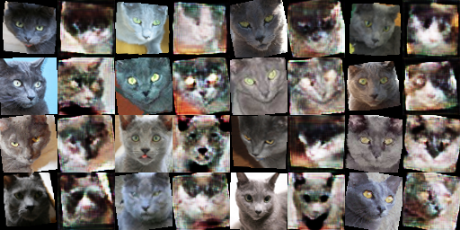
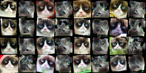
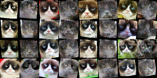
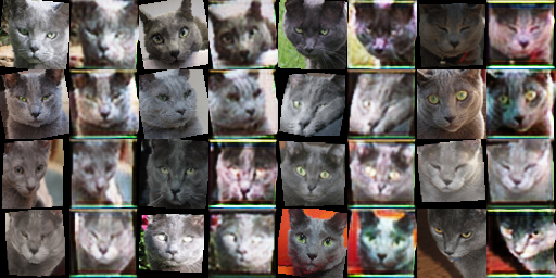
After the training with learning rate = 0.0002, beta1 = 0.5, beta2 = 0.999, epoch = 500, batch_size = 16, I get the results as below. From left to right, they are generated image with basic data augmentation, with basic and differentiable data augmentation, with deluxe data augmentation, and with deluxe and differentiable data augmentation.
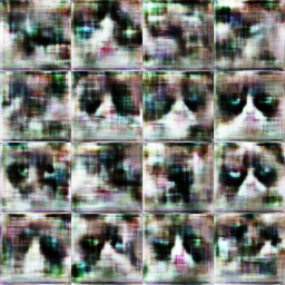
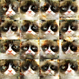
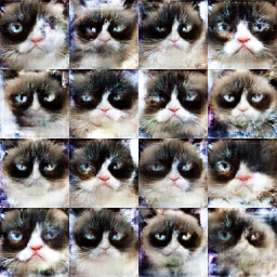
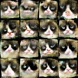
The result is interesting. It's obvious the basic method has a clumzy, hard to tell cat generation. And the differentiable method clearly has some color intensity and white balance shift, it actually proves the ability of this method to increase the robustness towards the RGB color intensity, and generate a more general color tone results, also it has a better recognition in the shape of cat. The deluxe result has a better detail than the differential method. And finally, the mix of deluxe and differential method is hard to tell if it's better than a single method, because some of the generation has both good detail and color tone but some are more blur or distorted, but if we only want one best result from a group of samples, this mix method definitely works better than either of the single method.
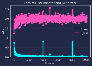
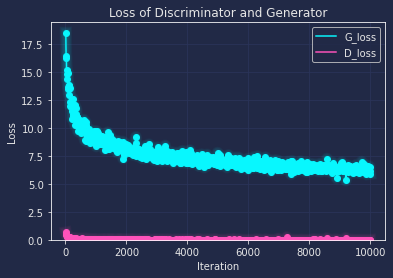
Similarly to the order above, I also draw the loss curve along with every 200 iteration as below:
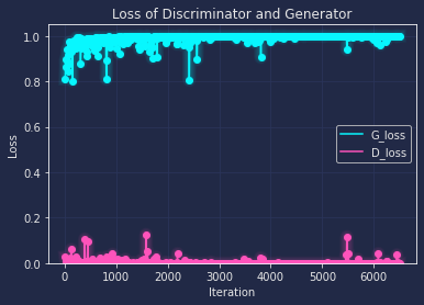
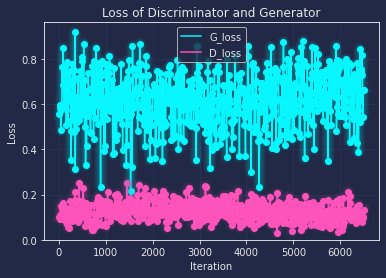
From the loss curve, we can tell that the base and deluxe both have the trend to overfitting after the training, though dexule has a relatively better loss(where G and D both are close to 0.5), and with the help of differentiable augmentation, the loss is more close to the ideal value, which means the network has a better robust performance on general data.
Part II: CycleGAN
The Dual Generator
The generator of CycleGAN is a convolutional neural network with the following architecture:
In the generator neural network, there are two generator for X->Y and Y->X, they are symmetric in input and output, and their architecture are identical in this project. The filter size is the same as in DCGAN, refer to them in convolution and upconvolution layer respectively. And one major difference is the ResnetBlock, which is used 3 times here, which aims to make sure characteristics of the output image (e.g., the shapes of objects) do not differ too much from the input. One major difference of this generator from the one of DCGAN is that its input is not noise anymore but an image.
The PatchDiscriminator
A major difference of this PatchDiscriminator from the Discriminator of DCGAN is that its output is a 4x4 patch instead of a loss value, which means the output layer doesn't require a softmax function anymore, and the rest are pretty much the same.
The Training Loop
The training loop including loss function and backpropagation is as straight forward as image below:
The major loss function and pipeline are similar to DCGAN, except for that for generator, since we have two generators, and we want to train them at the same time, so we add both X->Y and Y->X loss here; And for the discriminator, it goes the same way to train the loss from fake images generated from X->Y and Y->X.
The Cycle Consistency
The cycle consistency is like the soul part of the CycleGAN from my own experience of experiment, it aims to
The CycleGAN Experiments
My training for CycleGAN follows the learning rate = 0.0002, beta1 = 0.5, beta2 = 0.999, batch_size = 16 same as DCGAN, and I always use the Differentiable Augmentation since it helps increase robustness towards the RGB intensity and other factors. I first start by testing the CycleGAN with epoch = 1000, with and without cycle consistency, and the results are(Left side are without cycle, right side are with cycle; up side are X->Y, down side are Y->X):
It's clearly that 1000 epoch is not enough to get a good output, but from the basic shape of it, and the loss function below, we can tell that the general direction is good to extend the epoch.(Left without cycle, right with cyckle) And we can tell that the cycle consistency has a slightly better output.
Next I extend the epoch to 10000, and train the CycleGAN with two datasets, also I made comparison that with and without cycle consistency, patchDiscriminator and DCDiscriminator. The result are listed below:(Left is patch+cycle, middle is patch no cycle, right is dc+cycle)
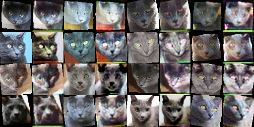
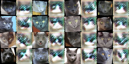
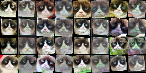
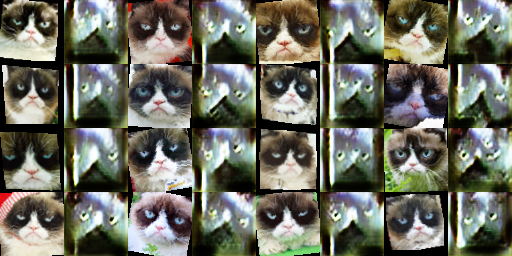
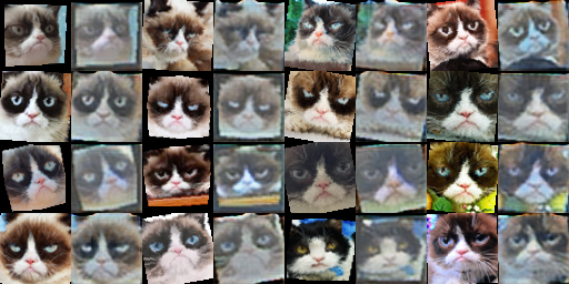
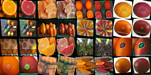
By observing the results above, we can see that without cycle consistency(middle column), the generated results have weird color, unclear shape. And for the DCDiscriminator(right column) and PatchDiscriminator(left column), they both achieve a relatively good result that generated fake image assembles the real image a lot. And they both have this color re-mapping effect, by comparison, I think the PatchDiscriminator has a slightly stronger color shift in all interested regions. It means that PatchDiscriminator can perform better pattern rematch effect.
Bonus
Extra dataset
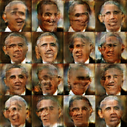
I choose one dataset from https://data-efficient-gans.mit.edu/datasets/ to apply to DCGAN, the output is like:
Assignment #4
Lorem ipsum dolor sit amet, no eum reque putent scripta. Eos esse vidit nonumy eu. Sit ut nominati prodesset, affert consul expetendis et cum. Sea cu animal cotidieque. Ei qui affert voluptua hendrerit, eripuit menandri pericula et per. Eam cu iusto possim vocent, veri mazim sensibus ea has, salutandi periculis his eu. Mei tractatos sententiae no. Eu vim eirmod molestie electram, eam ad dicunt facilisi conclusionemque, at nostrud delectus incorrupte mea. Vel ea liber munere maluisset, cu habeo cotidieque vel, blandit indoctum ei vel. Sit invidunt erroribus ne. Ea postea possit persecuti qui, tota dicit discere ut usu. Mei te iudicabit repudiare. Legere tritani definitiones vix ei, mea ea eros singulis. Qui ne posidonium definitionem, maluisset repudiare appellantur eam et, vim et vivendum facilisi delicatissimi. Ius ei choro dictas. Sit in atqui antiopam, ut his iuvaret oportere sapientem. Solet equidem recteque eum at, nam mundi perpetua te. Eum te semper appareat omittantur. Labitur perpetua ea mea, nam ea impetus partiendo. Elitr perfecto adipisci ut eum, his vocibus tincidunt incorrupte et. Ad duo putant tractatos. Sint case qualisque vis cu, soluta percipitur eu eam, cum inermis definitionem cu. Ne summo democritum pri, et falli ludus eruditi nam. Per assum mucius ex, no nec petentium delicatissimi, et pri hinc tacimates similique. Purto prima omnes vel ad, eu feugiat nostrum eum, ut has idque laoreet periculis. Ad vel officiis lucilius accusata, nonumy volutpat te qui. Noster indoctum mediocritatem ne cum.
Assignment #5
Lorem ipsum dolor sit amet, no eum reque putent scripta. Eos esse vidit nonumy eu. Sit ut nominati prodesset, affert consul expetendis et cum. Sea cu animal cotidieque. Ei qui affert voluptua hendrerit, eripuit menandri pericula et per. Eam cu iusto possim vocent, veri mazim sensibus ea has, salutandi periculis his eu. Mei tractatos sententiae no. Eu vim eirmod molestie electram, eam ad dicunt facilisi conclusionemque, at nostrud delectus incorrupte mea. Vel ea liber munere maluisset, cu habeo cotidieque vel, blandit indoctum ei vel. Sit invidunt erroribus ne. Ea postea possit persecuti qui, tota dicit discere ut usu. Mei te iudicabit repudiare. Legere tritani definitiones vix ei, mea ea eros singulis. Qui ne posidonium definitionem, maluisset repudiare appellantur eam et, vim et vivendum facilisi delicatissimi. Ius ei choro dictas. Sit in atqui antiopam, ut his iuvaret oportere sapientem. Solet equidem recteque eum at, nam mundi perpetua te. Eum te semper appareat omittantur. Labitur perpetua ea mea, nam ea impetus partiendo. Elitr perfecto adipisci ut eum, his vocibus tincidunt incorrupte et. Ad duo putant tractatos. Sint case qualisque vis cu, soluta percipitur eu eam, cum inermis definitionem cu. Ne summo democritum pri, et falli ludus eruditi nam. Per assum mucius ex, no nec petentium delicatissimi, et pri hinc tacimates similique. Purto prima omnes vel ad, eu feugiat nostrum eum, ut has idque laoreet periculis. Ad vel officiis lucilius accusata, nonumy volutpat te qui. Noster indoctum mediocritatem ne cum.