Gradient Domain Fusion
CMU 16-726 Image Synthesis S22
Tomas Cabezon Pedroso
In this project, we will exprole gradient-domain processing, a simple technique with a broad set of applications including blending, tone-mapping, and non-photorealistic rendering. For this assigment, we will focus on 'Poisson blending', 'mixed gradients' and 'color2gray'.
The primary goal of this assignment is to seamlessly blend an object or texture from a source image into
a target image. The method presented above is called “Poisson blending” and uses the gradients of both
of the images that we want to combine to make transition as smooth as possible. This was introduced by
Perez et al. in this 2003 paper.
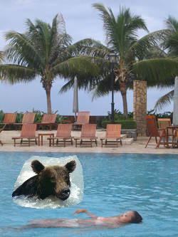
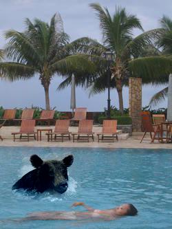
In the previous image, in the left, we have the target image, in which we want to add another image,
what we will
call, the source image, in this case, a bear. Next to it, we have the naive blend, a simple
copy and paste using a mask. This however, doesn't give good result, therefore, on the right, Poissong
blending has been applied.
Process
Gradients
To understand Poisson, blending, first we need to understand what a gradient is. As in calculus, a gradient is the derivative of a function, in this case, the derivative of each pixel. But how do we calculate this? To do so, we have to start by thiking what a derivative is: the rate of change of a function in a given direction. In the case of pixels, this is calculated by comparing the different values of the pixels in a given direction. Let's imagine the following 3x3 image with values for the each pixel of [[0, 1, 2],[3, 4, 5],[6, 7, 8]]. The derivatives of the p4 pixel will be defined by its 4 neighbours: p3 to the left, p5 to the right, p0 going up, and p7 going down. So the derivatives can be written as follow:
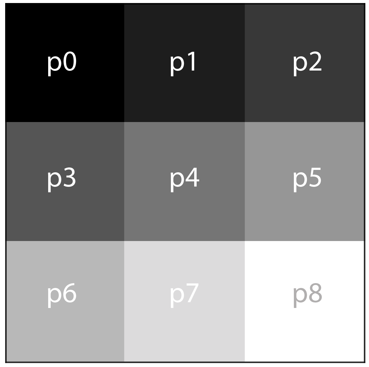
← p3-p4=3-4=-1
→ p5-p4=5-4=+1
↑ p1-p4=1-4=-3
↓ p7-p4=7-4=+3
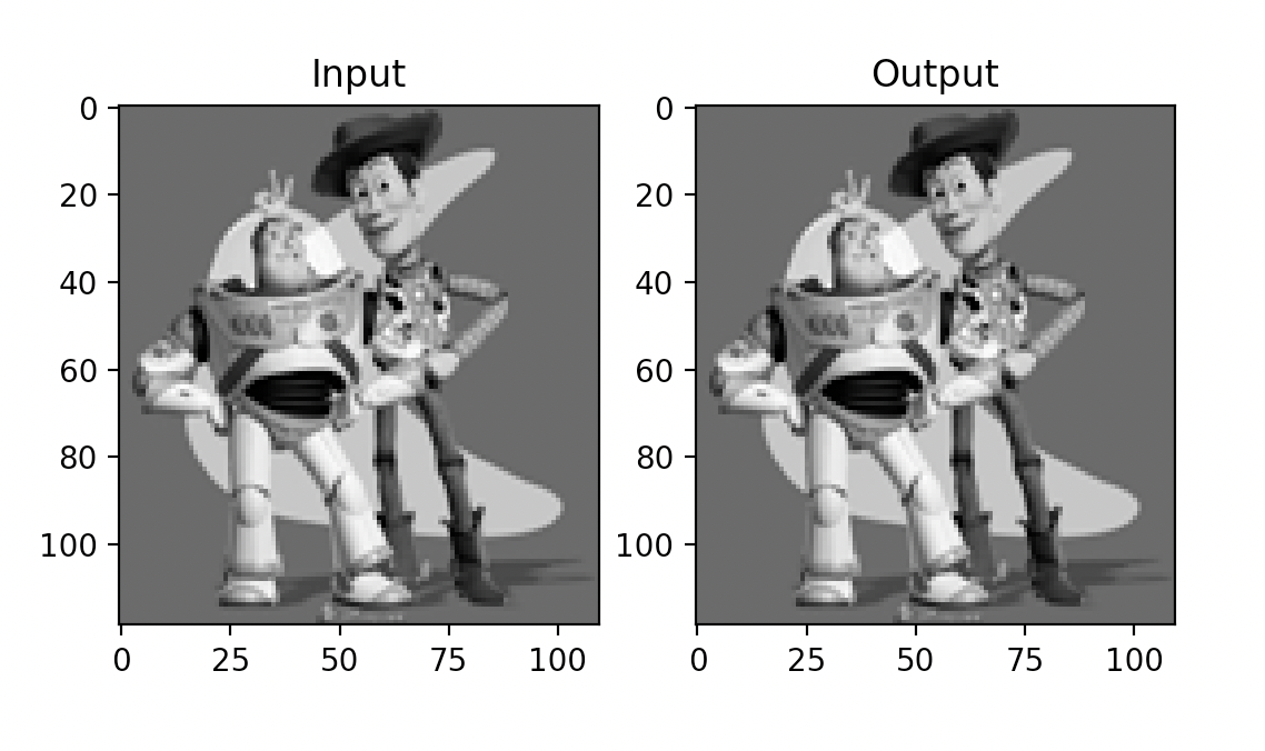
Toy problem
Before implementing the Poisson blending algorithm, we are asked to solve a toy problem. In this example we’ll compute the x and y gradients from an image s, then use all the gradients, plus one pixel intensity, to reconstruct an image v. If the implementation is correct, the output should recover the input image. Let's denote the intensity of the source image at (x, y) as s(x,y) and the values of the image to solve for as v(x,y). For each pixel, then, we have two objectives:
- Minimize ((v(x+1,y)−v(x,y))−(s(x+1,y)−s(x,y)))2, so the x-gradients of v should closely match the x-gradients of s.
- Minimize ((v(x,y+1)−v(x,y))−(s(x,y+1)−s(x,y)))2, so the y-gradients of v should closely match the y-gradients of s.
The result after minimizing the objectives:
Poisson blending
In order to make a seamless transition between any two images we need to think about the gradients of both of the images rather than about the overall intensity. This problem consists in finding the right values for the target pixels that maximally preserve the gradient of the source region, without changing any of the background pixels. Note that we are making a deliberate decision to ignore the overall intensity, so somo color change could occur, as seen before, a brown bear could turn black, but it would still look like a bear.

We can formulate our objective as a least squares problem. Given the pixel intensities of the source
image “s” and of the target image “t”, we want to solve for new intensity values “v” within the source
region “S”:

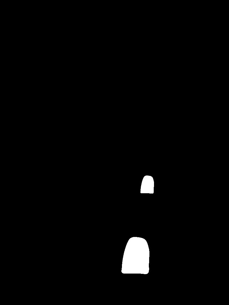
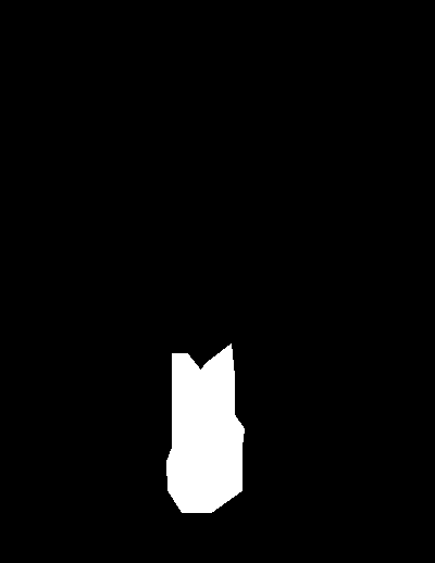
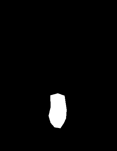
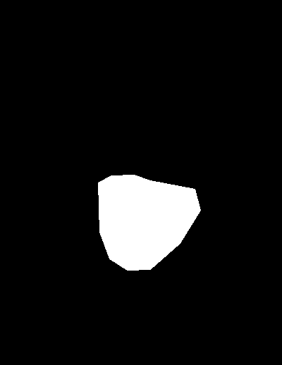
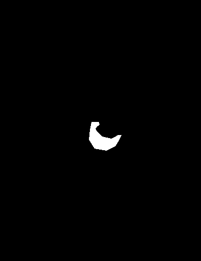
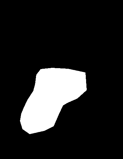
In the previous formula, we can see that we are summating the pixels of the region “S”. This region
represents the points of the source image that we want to copy in the target image. For this task, we
were given the following code, to create the mask and align it with both the source and target images.
In the formula,each “i” is a pixel in the source region “S”, and each “j” is a 4-neighbor of “i”. Each
summation
guides the gradient values to match those of the source region. In the first summation, the gradient is
over two variable pixels; in the second, one pixel is variable and one is in the fixed target region. In
the first part, we set the gradients of “v” inside "S" while on the second part, we set the gradients
around the boundary of “S".
To solve for v, we have used the scipy.sparse.linalg.lsqr function. This function minimizes our least
squares problem with the form of (Av-b)2. It returns the v values that minimize
the gradients and that are used to generate the output image.
Results
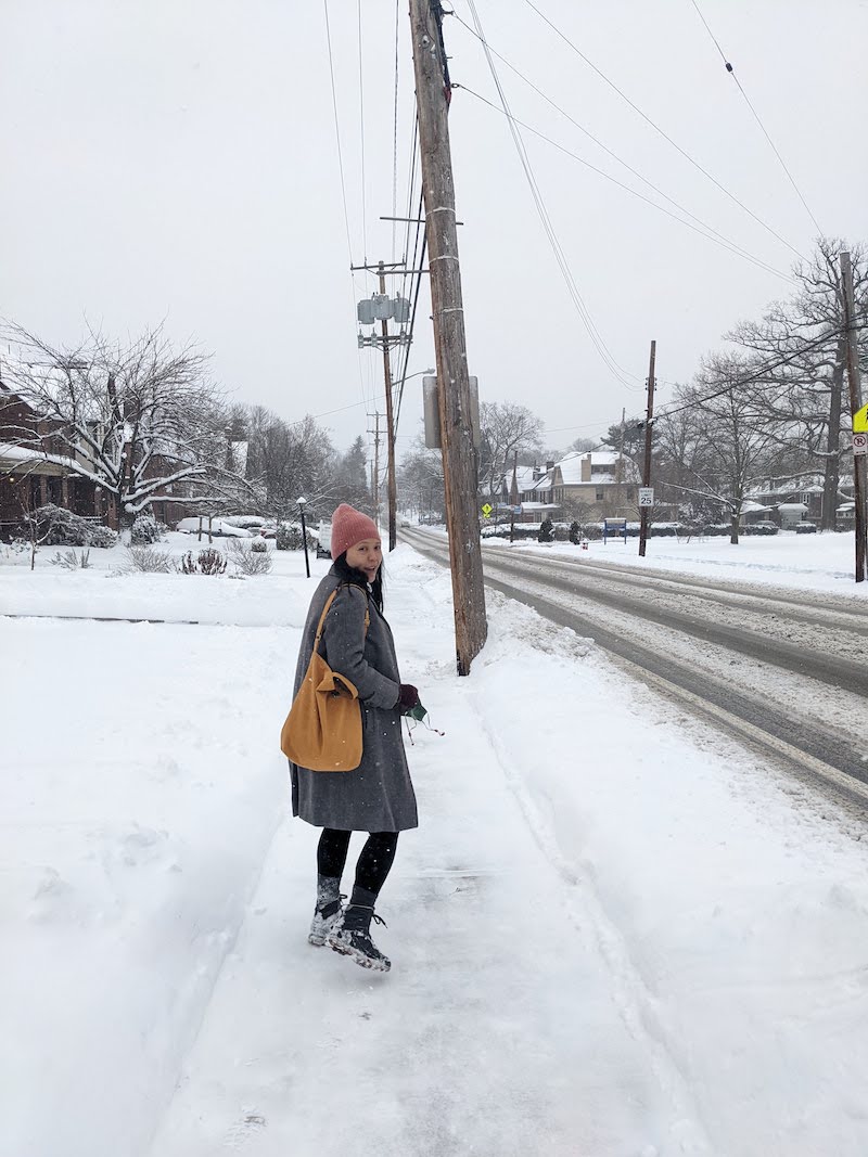
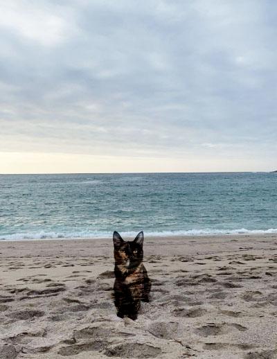
Kiki travels
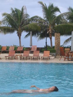
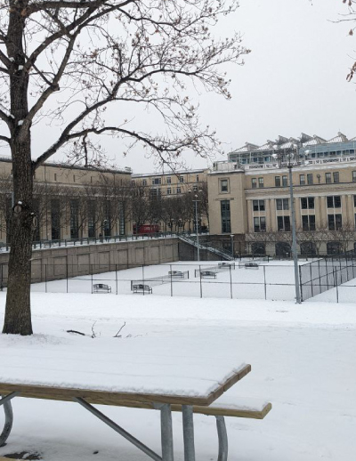
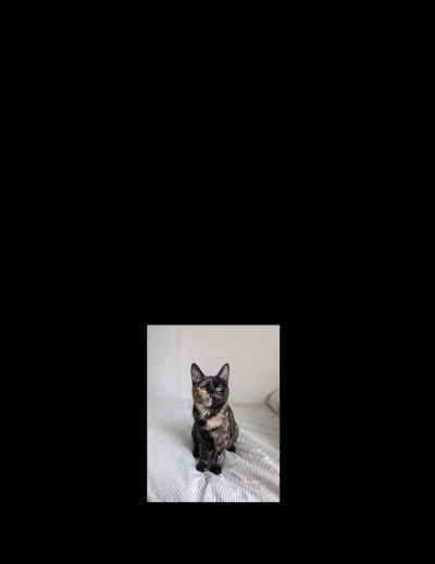
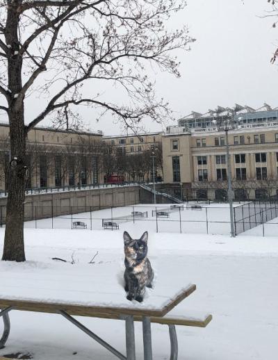
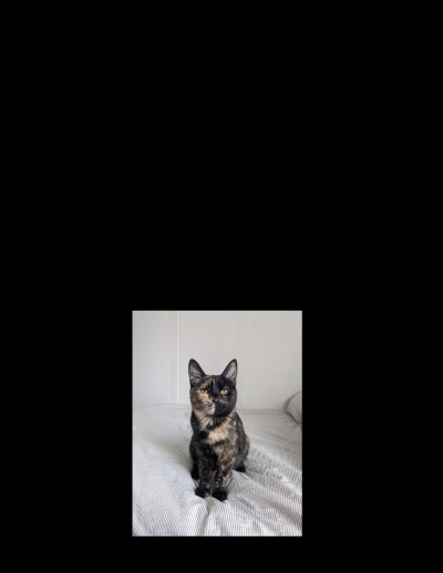
For this example I have tried to take Kiki, my cat, around so she can explore new places. I have used
the Poisson blending algorithm to take her with me to CMU on an snowy day. I have also taked her to the
beach, a place I could also take myself too...
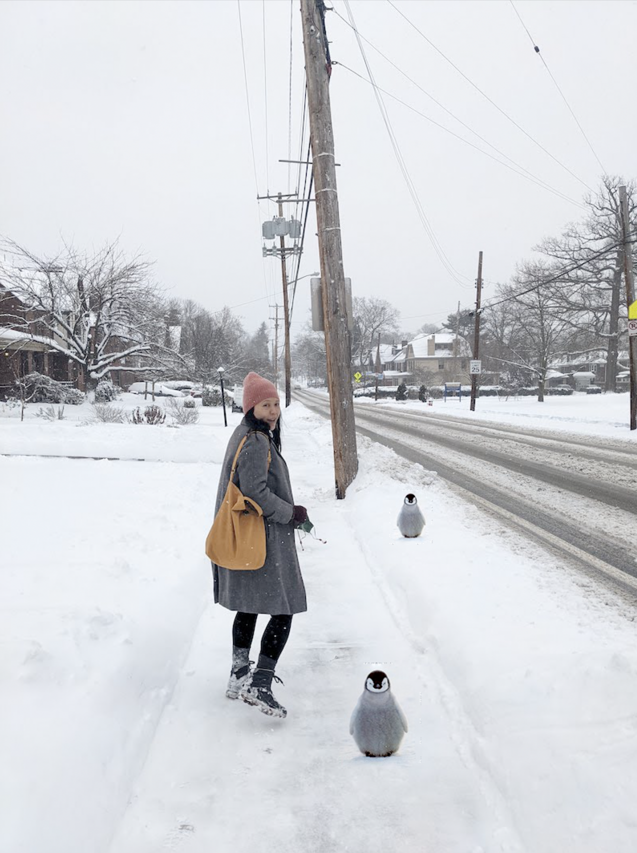
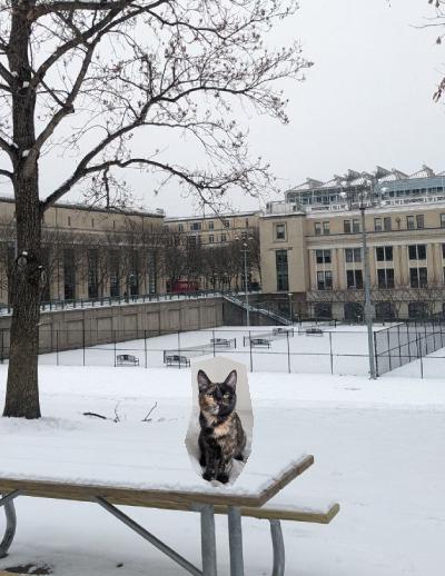
Kiki in CMU:
Kiki in the beach:
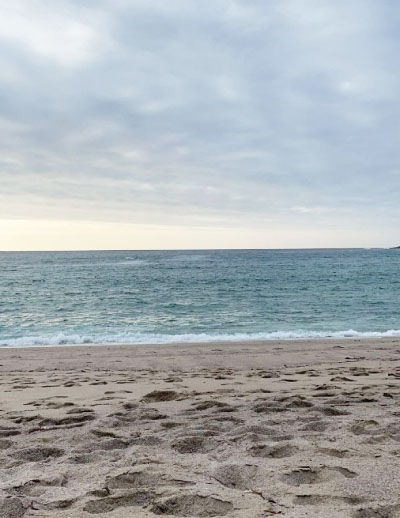
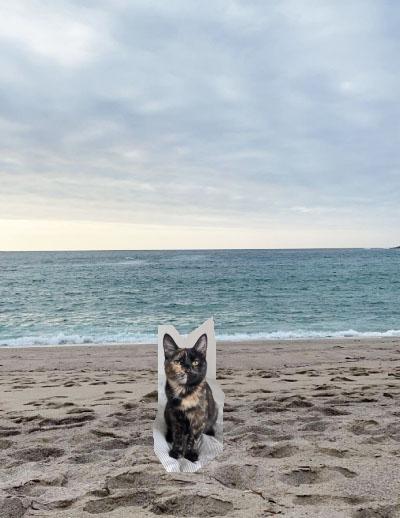
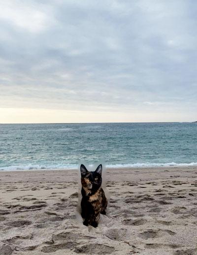
I am pretty surprised with the results! However, some artifacts can be seen in the image of Kiki at CMU. Between her ears the fence of the tenis court disappears. On the beach case, the output image makes Kiki too dark due to the gradients. Furthermore, the blending is not as good as in the previous image. This is because the background colors matched better in the previous example.
Naruto's Deidara
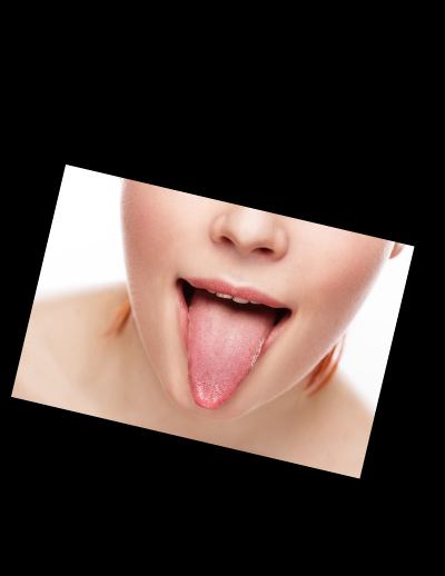
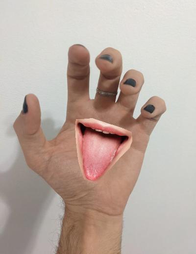
When I was young I used to read Naruto's comics. Back then I was a fan of one of the characters,
Deidara, that had mouths in her hands:
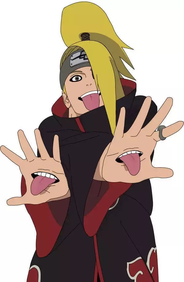
Using this algorithm I have been able to be like her, at least virtually.
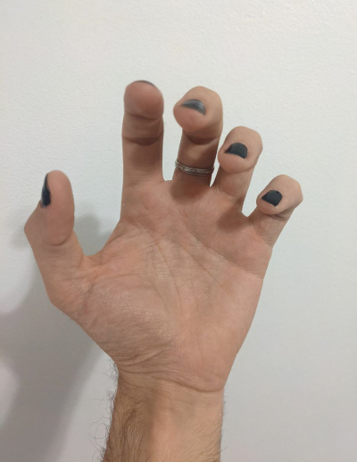
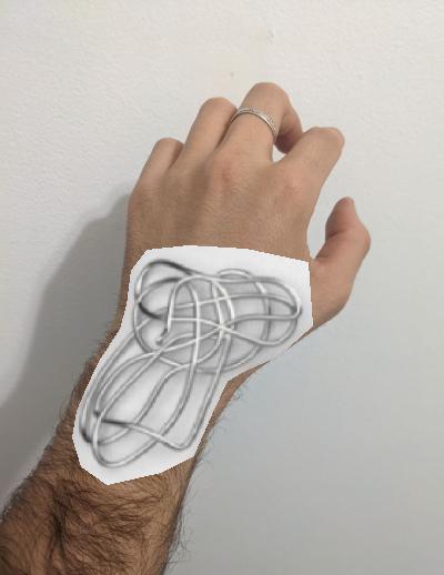
Trying jewelry
I really enjoy designing rings or other kind of wearables, so I thougt that this could be a great opportunity to inquire the possibilities of poisson blending algorithm for trying jewelry.
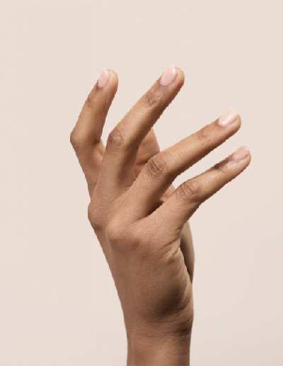
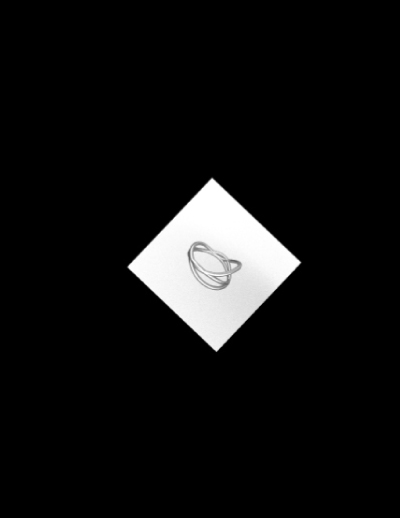
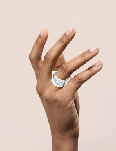
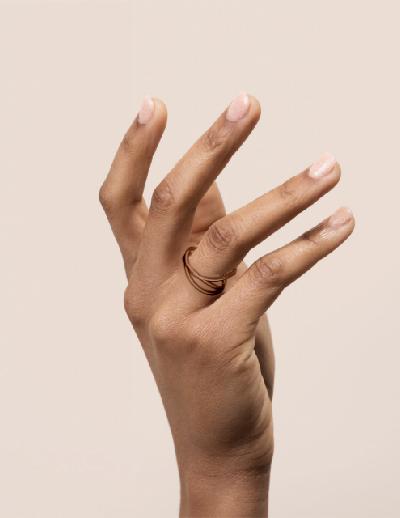
I think this is a great tool to create rapid mockup images whithout espending a lot of time on
making a perfect mask around the ring. In this example we can also see what we mentioned before, that
this algorithm changes the color of the objects. Actually, the color of the silver ring dissapears as it
fuses with the color of the skin.
After seeing this results, I wondered how this algorithm would
work with a more complex shape... so I tried it!
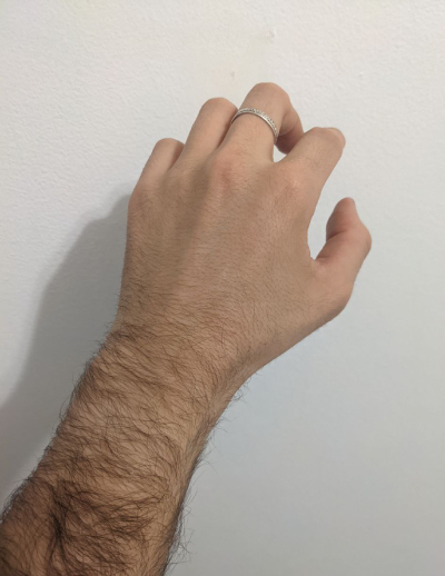
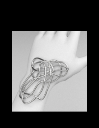
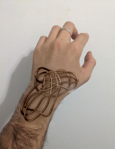
This time the results are not as surprising as before. Mainly because I lost all my hair in the procces due to the blending. To solve this problem, I applied the mixed gradients algorithm in the bells and whistles of this assigment.
Bells and Whistles
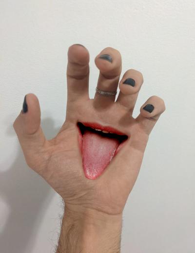
Mixed gradients
To solve the above seen problem, in this section we will implement the mixed gradients algorithm for
images where transparency important. In this algorithm we follow the same steps as in Poisson blending,
but
instead of using the gradients in the source image, we use the gradient with larger magnitude in either
source or target image as the guide:

The results of applying this algorithm to the previous image
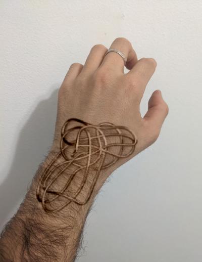
Mixed gradients works very well in this example. Nevertheless, this algorithm makes the source image too transparent. This is something we need to have into account when deciding which algorithm we are going to use. For example in the following images, we can see the results of applying mixed gradients to the Kiki goes to the beach image.
Although both of the images are seamlessly blended, when applying this algorithm, the source image may seem to became more transparent, is we zoom in, we can see that the beach can be seen thorugh Kiki's fur. This is because inside the region S, we now also consider the gradients of the target image.
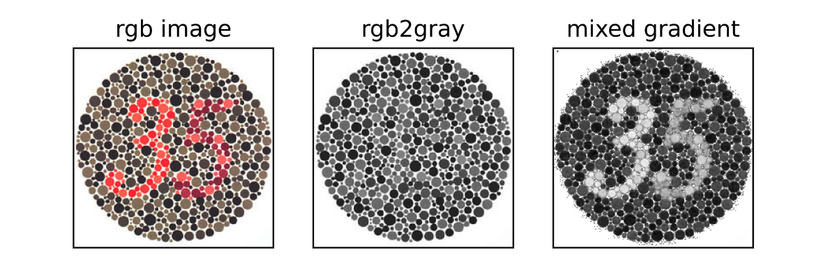
Color2gray
For this part of the assigment, we will see another application of these blending algorithms, color2gray
transformation. When converting a color image to grayscale (e.g., when printing to a laser printer), we
lose the important contrast information, making the image difficult to understand. To see this, we will
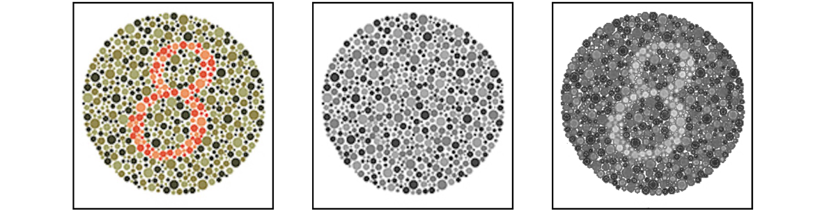
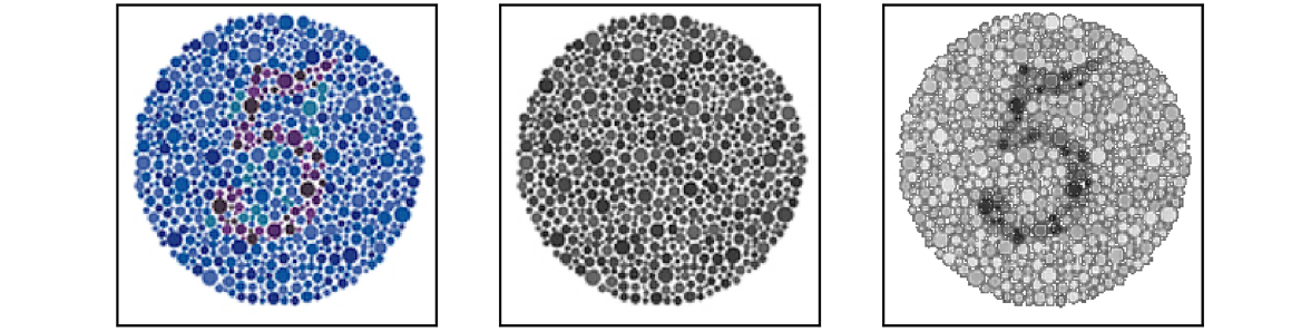
use the images used for testing color blindness. As it can be seen bellow, when this images are
converted into grayscale, no longer show the numbers. To solve this, we are going to use this blending
techniques to create a gray image that has similar intensity to the rgb2gray output but mantaining the
contrast of the original RGB image.
To do this, we first convert the RGB image into HSV(Hue Saturation Value) space. In the image bellow we
can see the example image as an RGB image on the left, and next to it the correspondent images of each
of the HSV channels.

In the HSV space, we can examine the color of an image, the intensity of that image and the brightness.
The image representing the brightness, is similar to the rgb2version. Therefore, to create our
color2gray version, we will use the S and V channels of the image and approach it as a mixed gradients
problem. We will use the white pixels of the original image to generate a mask. The results of this
color2gray: