Introduction

Vision-based robotic manipulation models often assume access to a goal image, i.e. how the scene would look if the ideal action plan is executed, then use this image and current observations to uncover the optimal plan [1, 2]. Even further, having the target image is important for autonomous robots, as they can compare their observations to the goal and decide whether they make progress or when they need to stop. However, for many practical open-ended cases where a robot has to generalize a behavior in different, perhaps novel, environments with different objects, expecting that a goal image is given is a very hard-to-satisfy assumption.

A possible solution to goal representation is to assume some task description in natural language, then use the language features to modulate the execution [3, 4]. This way, the language represents the goal implicitly and the different concepts it describes can be mapped to contrastive classifiers [5]. Another alternative is to generate the goal explicitly, either in the form of an image or a more abstract representation. Then, we can directly use our imagination of the goal i) to plan the next action and ii) to directly compare and be aware of the progress our actions contribute to.

In this work we ask the question, how can we explicitly generate useful explicit goal representations? A direct approach is to generate the goal image conditioned on the input and task description. However, in a manipulation setting we often care more about the relative deformation of objects and their pose, rather than exact pixel intensities. Moreover, while relations change following the abstract language descriptions, objects and (most of) their attributes persist in time. To address these challenges, we propose an object-centric image generation approach that i) learns both image and symbolic representations of individual object concepts, ii) uses the symbolic abstractions to synthesize relations, iii) uses the image generation modules to fill the abstracted templates and output a real image. For example, to generate “a green cube behind a yellow sphere”, we learn to represent each object as a box, then optimize these boxes wrt the relation (here “behind”) to get an abstract representation of the scene, and lastly we fill the slots of each object using a decoder that maps attribute latent vectors, e.g. [“green”, “cube”], to pixels. To optimize for the relative placement of boxes we use Energy-based models, while for rendering we use a convolutional generator. Our entity-based abstraction enables controllable graph-conditioned generation even when fewer data are used.

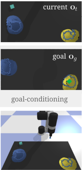
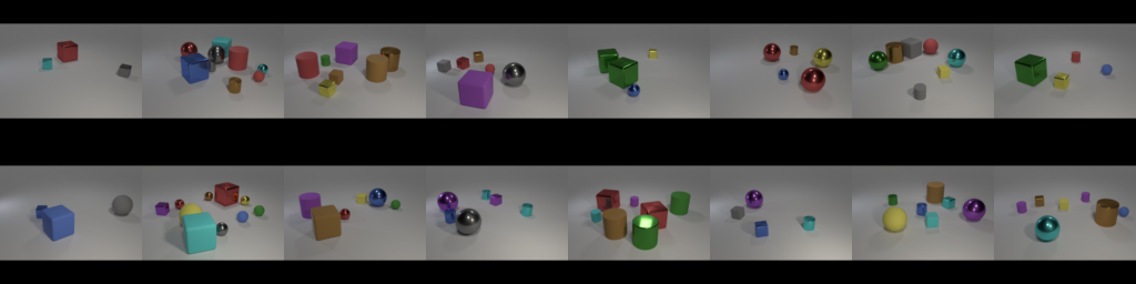
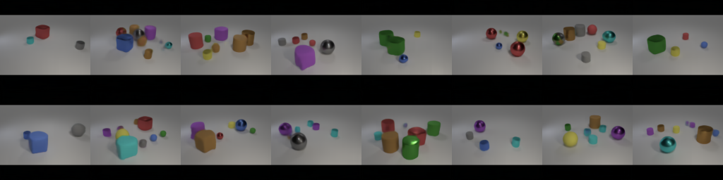
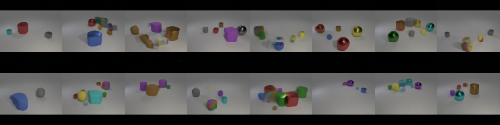
Robotic policies often rely on goal images. However, how to obtain these images in a new environment is not a trivial problem. We investigate image generation as a possible solution. Figure adapted from [1].

Related work

Image generation usually focuses on creating realistic images of high-fidelity. Most approaches use a holistic representation of the image, e.g. CNN/Transformer features [6, 7], and generate on the pixel level. A stream of those works focuses on manipulating images by editing their style or attributes [8]; still, those methods operate on image-wise features and rely on an abundance of training examples in order to implicitly learn disentangled representations. In general such a representation i) needs more data to learn a concept and ii) is not compositional, e.g. if we learn to generate a giraffe, it is still hard to generate three giraffes. Moreover, in robotics we care about manipulating a given scene, not generating one from scratch.

The recent work of Liu et al. [9] decomposes text-guided image generation into a joint optimization problem over different specialized modules that learn a specific concept. The tested hypothesis is that if we learn generative models over a vocabulary of objects, attributes and relations, we can then compose arbitrary scenes on-the-fly, by using the learned concepts as building blocks. For example, to generate “a blue cube behind a yellow sphere and a green cube left of a red cylinder”, their approach is to jointly optimize two energy-based models, one for “blue cube behind a yellow sphere” and one for “green cube left of a red cylinder”. This allows zero-shot generalization to previously unseen combinations of concepts.

However, [9] still operates on an image-wise representation: at test time, they start from random noise and optimize the input. Given the desired combination of energy-based models, the input is updated by summing its gradients as computed by each model. We find that this is suboptimal for two reasons. First, by generating pixels we lose an important level of abstraction: many relation primitives, especially the spatial ones, can be adequately represented as bounding boxes with attributes. Second, if we optimize image latents, we do not have control over implicit graphs of relations. For example, let A, B and C be some object descriptions and we want to optimize for “A left of B and right of C”. The method of [9] would decompose this into “A left of B” and “A right of C”, then it would optimize the input image jointly for these two relations. However, this optimization ignores the fact that A refers to the same instance in both sentences: the model is free to generate an image with an instance of A left of B and another instance of A right of C. Instead, we jointly optimize on entities, thus handling graphs of relations, as opposed to solely lists that [9] supports. This allows for better disentanglement and control.

Energy-based models (EBMs): [10] are a family of generative models that iteratively optimize the input $x$ so that it is consistent with a desired concept description or label $y$. The compatibility of $x$ and $y$ is parametrized by a scalar energy value. At test time, we can optimize over the sum of energy values for joint satisfaction of otherwise independent concepts. EBMs have been applied both on images [9] as well as on abstract representations [11]. Some tricks we also use to improve convergence are discussed in [12].

Two-stage generation: approaches that go through an intermediate representation are also relevant to this work. For example, [13] first generates a semantic map and then conditions on it to render details. We use box abstractions for our domain, but we could also extend it to generate masks, which could handle deformable objects as well.

Approach

Our pipeline is shown in the following architecture figure. We assume that a scene description is already decomposed into a scene graph, where each node is an object with known attributes. Then, we jointly optimize over the object boxes so that they satisfy the scene graph constraints. For each visual relation, i.e. (obj$_1$, rel, obj$_2$) triplet, we compute and energy. We minimize the sum of energies. In the next step, we render the image. This is achieved by feeding the encoded graph into a Transformer to get a latent vector, then feeding this into an image generator. The concept EBM and the render network are trained separately. We now dive into our architecture in more detail.

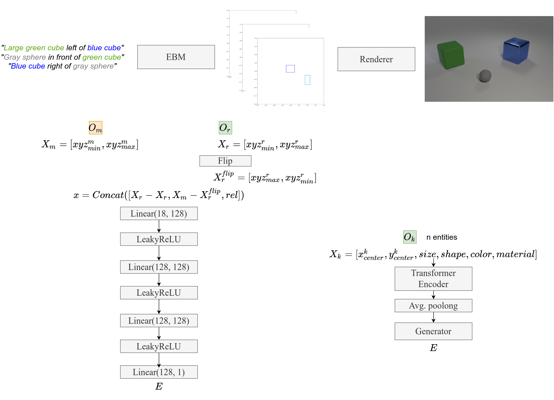
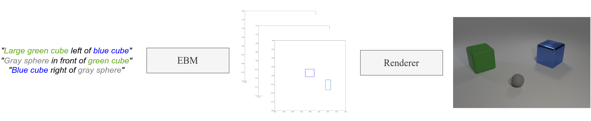
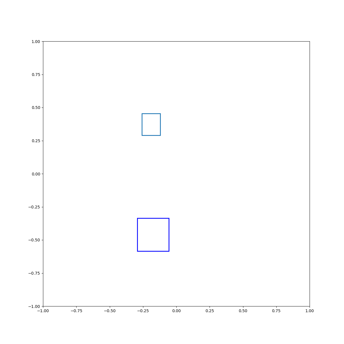
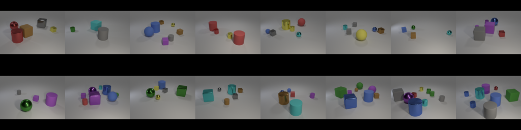
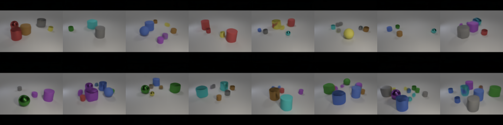
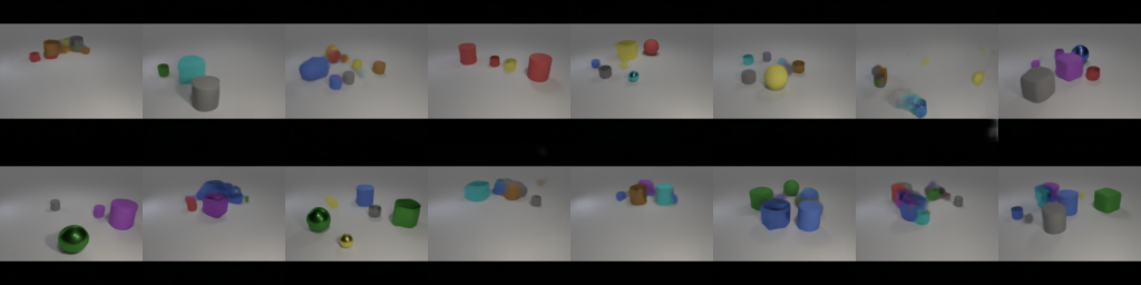
Upper: Full pipeline of our model. The input is a language scene graph that is converted to abstract symbolic representations which are fed into a rendering model to output an image. Bottom left: The architecture of the Concept EBM that maps graphs to boxes. Bottom Right: The architecture of the rendering module which maps object-centric graphs to images.

Relation concept learning: Energy-Based Models (EBMs) are a family of networks that output a scalar energy value $E_{\theta}(x)$ which measures the compatibility of the input $x$ and some constraints. Inspired by physics, where stable systems lie on smooth local optima of an energy function, the smaller the EBM output, the better the input satisfies the imposed constraints. During training, the EBM learns the positive data distribution $p_{\theta}(x) \propto e^{-E_{\theta}(x)}$ by minimizing the loss \begin{equation} \mathcal{L} = \mathbb{E}_{x^{+} \sim p_D}E_{\theta}(x^{+}) - \mathbb{E}_{x^{-} \sim p_{\theta}}E_{\theta}(x^{-}) \end{equation} where $x^{+}$ is a positive sample for the true data distribution $p_D$ and $x^{-}$ a negative sample drawn from the learned distribution $p_{\theta}$. To sample from $p_{\theta}$, we start from an initial estimate $x^0$ and refine using Langevin Dynamics [14]: \begin{equation} x^{k+1} = x^{k} -\lambda \nabla_x E_{\theta}(x^{k}) + \epsilon * noise \end{equation} After $K$ iterations, we obtain $x^{-}=x^{K}$. This formulation is intuitive: we follow the EBM's gradients wrt to the input to update the input in a way that minimizes the energy. These artificially good samples are treated as negatives. At convergence, the EBM is able to produce very realistic "negatives" using the above equation.

To incorporate the above formulation into our problem, we use a relational network that is shown in the architecture figure. The input is a pair of bounding boxes and a relation code. We compute relative features by subtracting the coordinates of the corners of the two boxes. The relation is represented as an one-hot vector. Then, we use a multi-layer perceptron (MLP) to output a scalar energy evalue.

We train the EBM on single visual relations. During training, we sample positive examples from the dataset, i.e. triplets labeled with the target relation, while the negatives are computed by following the gradients of the model. We pick $K=30$, $\lambda=1$ and $\epsilon=0.005$. Additionally, we employ the techniques of [12] to improve stability and convergence. Specifically, we use a replay buffer and a KL-loss term. The replay buffer stores previous negatives, which we sample as initializations. The KL-loss term encourages the network to assign low energy values on good-looking negatives.

During inference, we can compose energies of visual relations to obtain energies of graphs. Specifically, we initialize the boxes of each node in the graph. Then for each triplet, we compute the energy. We then sum the computed energies of all triplets and use this as $E_{\theta}$. This updates all boxes jointly so that they satisfy all constraints. At the same time, each node is associated with exactly one box, ensuring persistence and uniqueness.

Rendering: Once we have a graph representation with boxes and attributes, we encode everything into a latent vector and train a generator, which is depicted in the architecture figure. Each node is encoded by concatenating five types of learnable embeddings: size, color, material, shape and location. The concatenated vectors are projected to a lower dimension using a linear layer and are then fed into a Transformer to obtain a contextualized representation. We average over the nodes to get a scene latent vector. This is used to condition a generation network inspired by FastGAN [15] and modified to output images of 128 pixels at each dimension.

This network is trained on the ground-truth graphs that describe the training scenes. Since we know both the input and the expected output, we directly supervise with an L1 regression loss. All training scenes are used here. At test time, we feed the graphs the EBM outputs.

Results

We train and test our networks on CLEVR [16], which offers scene graph annotations on a domain related to a manipulation setup. We cannot directly use the dataset of [9], as they do not offer box annotations.

First we evaluate the accuracy of the graph generation on a relation-level and a graph-level. The former measures how many relations can be correctly classified by an oracle classifier. The former measures the percentage of images for which all relations are classified correctly. The results are shown in Table 1. Even with 1% of the training data we are able to maintain a high accuracy per relation. However the graph-level accuracy is low, but this is expected since it is a very strict metric. Note that we use dense scene graphs for CLEVR, which have 3-10 nodes and more than 75 edges on average. Although some of these relations are redundant, e.g. both “A left of B” and “B right of A” are annotated, this is a very constrained setup and makes joint energy optimization challenging. For comparison, [9] reports 37.6% accuracy when optimizing for 3 relations. This highlights the advantages of abstract object-centric generation.

Table 1: Relation classification accuracy on generated images

Method	Relation acc	Graph acc
CLEVR Full	84.5	6.9
CLEVR 1%	75.8	1.0

We visualize the generative process in the following gifs. Here we move the light blue box to be left/right respectively from the navy blue one. Note that our model is not trained on trajectories but instead simply scores images. Training and optimizing with Langevin dynamics creates a smooth energy landscape where a solution can be found by following a trajectory towards a local minimum. Also note that our EBM operates on 3D boxes, but we show the 2D projection here for clarity.

Lastly, we evaluate the rendering capability. Rendering with ground-truth graphs achieves very good reconstruction of the scene. A common mistake is that cubes often appear as cylinders. This is because the relative is not explicitly modeled. When using predicted graphs, the outputs are usually compatible with the descriptions and the initial scene, although the relative placement is always different. Scenes with more objects and thus more occlusions are generally harder to generate. The FID scores in Table 2 reflect that difference.

Table 2: FID scores for rendering under different graph models

Method	FID
GT graphs	99
Predicted graphs	144
Predicted graphs 1%	175

Qualitatively, a comparison between the ground-truth scenes, the scenes rendered using ground-truth graphs and the ones rendered with predicted graphs are shown below. In most of the cases, with predicted graphs we are able to render high-quality images that respect most of the relations in the original image, as well as the number of object nodes. Scenes with many objects and occlusions are the hardest to replicate.
Original image:

Reconstructed with ground-truth graphs:

Rendered with predicted graphs:

Original image:

Reconstructed with ground-truth graphs:

Rendered with predicted graphs:

Conclusions and Future Steps

Motivated by goal imagination in robotics, we tackle the problem of controllable image generation under graph constraints. From a robotics perspective, the concept EBM is able to explicitly model goal configurations in an abstract space, which can be used to modulate action plans. At the same time, it can compose an arbitrary number of constraints by joint optimization with high accuracy, despite being trained only for a single relation at a time. This decomposition of concepts and constraints allows us to learn fast, even from 1% of the annotations. Then, from an image generation perspective, we learn a rendering model that is optimized over scene graph latent vectors. The renderer has to map a graph into a scene and is agnostic to relations, thus reusable even if the vocabulary of relations changes.

A limitation of our approach is that the abstraction scheme we adopt is peculiar to a domain. While we expect bounding boxes to generalize to standard manipulation setups, the representation with boxes is insufficient for general cases, such as visual relations between deformable objects in real-world images. While previous literature has shown that segmentation masks can be a good intermediate representation [13], identifying the right level of abstraction for each task remains an open question.

References

[1] Daniel Seita, Pete Florence, Jonathan Tompson, Erwin Coumans, Vikas Sindhwani, Ken Goldberg, Andy Zeng. Learning to Rearrange Deformable Cables, Fabrics, and Bags with Goal-Conditioned Transporter Networks. ICRA, 2021

[2] Thomas Weng, Sujay Bajracharya, Yufei Wang, Khush Agrawal, David Held. FabricFlowNet: Bimanual Cloth Manipulation with a Flow-based Policy. CoRL, 2021.

[3] Corey Lynch, Pierre Sermanet. Language Conditioned Imitation Learning over Unstructured Data. RSS, 2021.

[4] Mohit Shridhar, Lucas Manuelli, Dieter Fox. CLIPort: What and Where Pathways for Robotic Manipulation. CoRL, 2021.

[5] Alec Radford, Jong Wook Kim, Chris Hallacy, Aditya Ramesh, Gabriel Goh, Sandhini Agarwal, Girish Sastry, Amanda Askell, Pamela Mishkin, Jack Clark, Gretchen Krueger, Ilya Sutskever. Learning Transferable Visual Models From Natural Language Supervision. CVPR, 2019.

[6] Alec Radford, Luke Metz, Soumith Chintala. Unsupervised Representation Learning with Deep Convolutional Generative Adversarial Networks. Arxiv, 2021.

[7] Aditya Ramesh, Prafulla Dhariwal, Alex Nichol, Casey Chu, Mark Chen. Hierarchical Text-Conditional Image Generation with CLIP Latents. ArXiv, 2022.

[8] Tero Karras, S. Laine, and Timo Aila. A style-based generator architecture for generative adversarial networks. CVPR, 2019.

[9] Nan Liu, Shuang Li, Yilun Du, Joshua B. Tenenbaum, Antonio Torralba. Learning to Compose Visual Relations. NeurIPS, 2021.

[10] Will Grathwohl, Kuan-Chieh Wang, Jorn-Henrik Jacobsen, David Duvenaud, Mohammad Norouzi, Kevin Swersky. Your classifier is secretly an energy based model and you should treat it like one. ICLR, 2020.

[11] Igor Mordatch. Concept learning with energy-based models. ICLR Workshops, 2018.

[12] Yilun Du, Shuang Li, J. Tenenbaum, Igor Mordatch. Improved contrastive divergence training of energy based models. ICML, 2021.

[13] Drew A. Hudson, C. Lawrence Zitnick. Generative Adversarial Transformers. ICML, 2021.

[14] Max Welling and Yee Whye Teh. Bayesian learning via stochastic gradient langevin dynamics. ICML, 2011.

[15] Bingchen Liu, Yizhe Zhu, Kunpeng Song, Ahmed Elgammal. Towards Faster and Stabilized GAN Training for High-fidelity Few-shot Image Synthesis. ICLR, 2021.

[16] Justin Johnson, Bharath Hariharan, Laurens Van Der Maaten, Li Fei-Fei, C Lawrence Zitnick, Ross Girshick. Clevr: A diagnostic dataset for compositional language and elementary visual reasoning. CVPR, 2017.