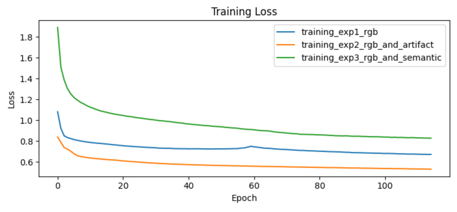
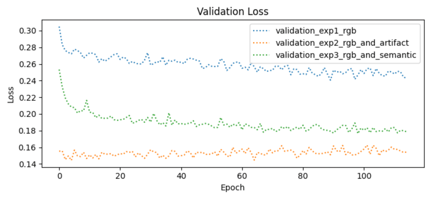
16-726: Learning-based Image Synthesis

Final Project: Semantics-Driven View Synthesis

Ingrid Navarro-Anaya (ingridn), Suann Chi (suannc)

1. INTRODUCTION

In recent years, research communities within fields like embodied AI, computer vision and natural language processing have envisioned designing agents that operate in environments that may be partially known and where human collaboration may be required. To achieve this, it is important that such agents are equipped with mechanisms that allow them to understand semantic contexts of an environment. One way to extract and understand semantics includes leveraging and aligning information from sensory inputs, including: visual images, masks, audio, language, motion, etc. Toward this challenging objective, we are interested in studying how we can align explicit semantic information with visual and motion information to learn to represent 3D structure and ego-motion from monocular vision.

Specifically, we aim to explore the task of view-synthesis as a methodology for learning to represent 3D structure and ego-motion from monocular vision. Previous research in view synthesis has shown that models can be trained to generate reasonable ego motion outputs given video inputs from car dashboards (i.e. the KITTI dataset [7]) [6]. In this study, a pose and explainability network in conjunction with a depth network was used in order to generate a 3D video prediction of the dashboard video. Other research employs semantics-driven unsupervised learning in order to train their ego-motion estimation models [8].

Our project, SemSynSin (Semantics-driven ViewSynthesis from a Single Image), builds on these ideas in order to generate ego motion videos from indoor scenes.

The sections that follow are organized as follows:

  • In the Approach section, we discuss the approach we take in order to generate indoor ego motion videos. For this project, indoor scenes from the MatterPort3D dataset were used. Additionally, trajectory information from the Vision-Language Navigation dataset was used.
  • In the Experiments section, we describe the ablation experiments under which we test SemSynSin.
  • In the Results section, we show the results generated by the SemSynSin model under the different experimentation conditions.
  • In the Discussion section, the results of SemSynSin are discussed, as well as potential avenues of future research.

2. APPROACH

In this project, we are interested in learning the 3D structure of complex indoor environments via view-synthesis. View synthesis allows generating images of a scene from different viewpoints. This is a highly challenging task as it requires developing algorithms capable of understanding the nature of 3D environments, e.g., the semantic information in a scene, the relationship between objects in a scene, and the layout of environments and occlusions.

As mentioned above, we build on prior work which focused on learning Structure-from-Motion (SfM) from single-view images in outdoor environments. We first asses the model's performance on complex indoor environments, and then explore methods for improving the results. Particularily, we are interested in explicitly incorporating semantic knowledge since it is crucial for scene understanding.

In the following sub-sections, we further describe the procedure followed in this project. Specifically, in Part 1, we described our methodology for obtaining the training data. Then, in Part 2, we describe the model and the loss functions we used.

Here's the link to our project code.

2.1 The Dataset

We use the Matterport3D (MP3D) dataset for our project and the Habitat simulation environment to generate egocentric trajectories for training, validation and testing. This section describes in more detail the procedure followed to generate said dataset.

Figure 1. Matterport3D trajectory obtained through the Habitat simulation environment.

2.1.1 The Scenes

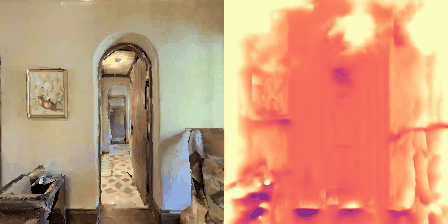
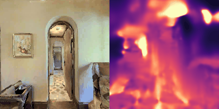
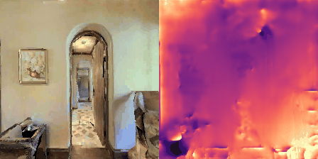
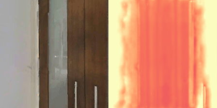
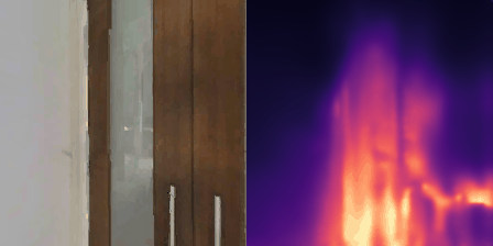
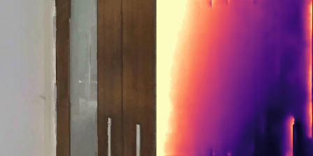
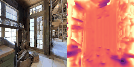
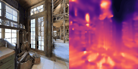
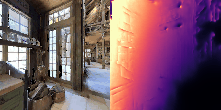
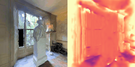
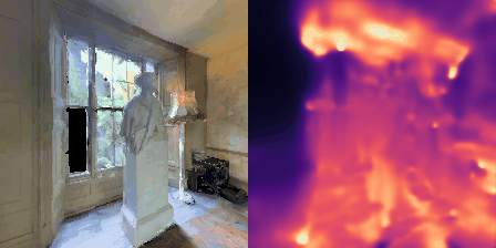
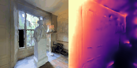
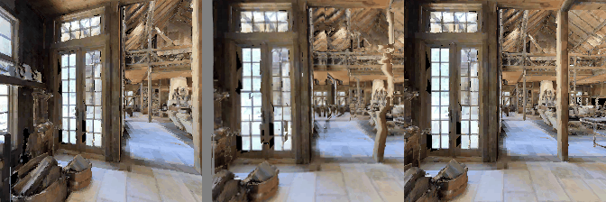
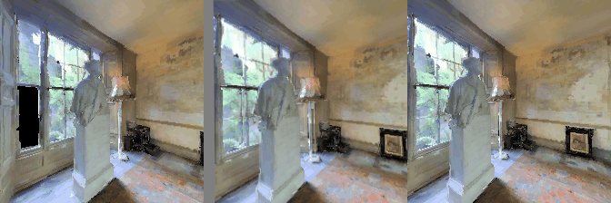
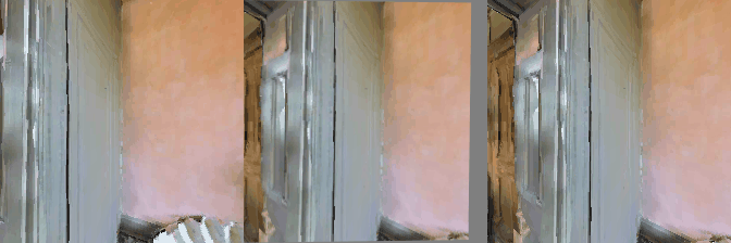
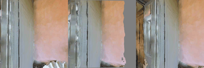
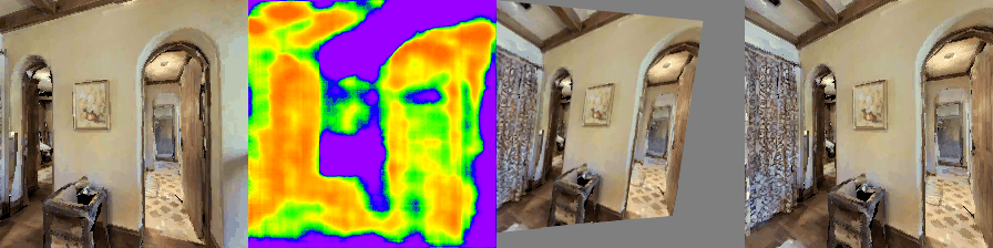
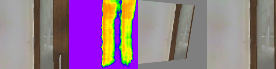
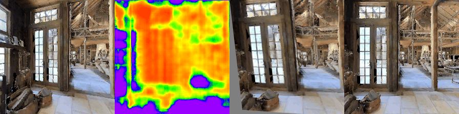
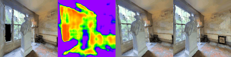
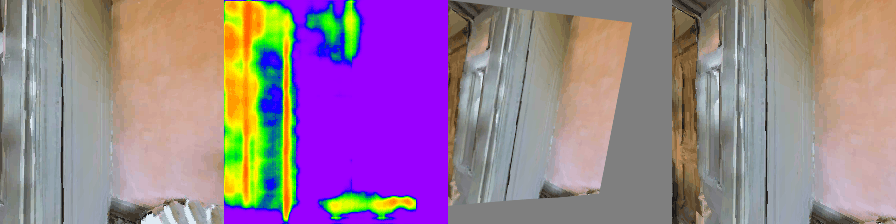
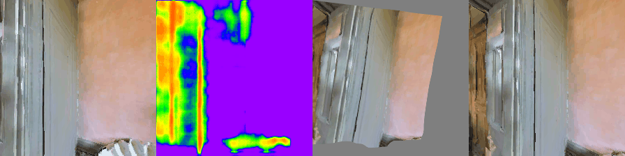
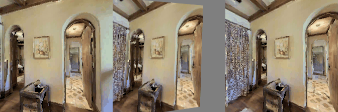
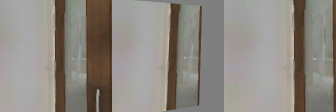
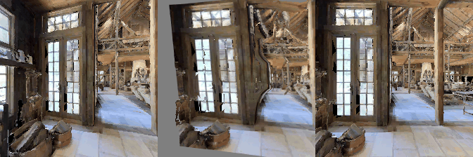
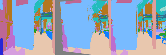
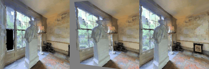
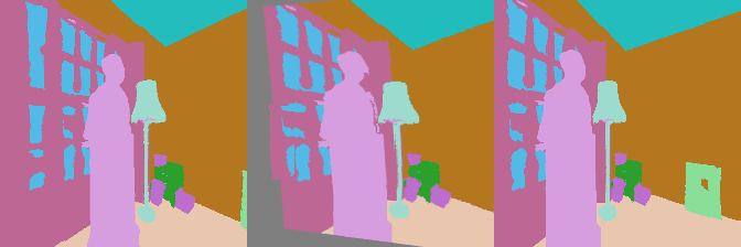
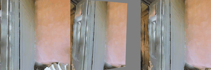
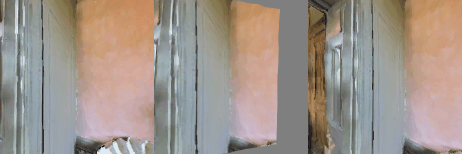
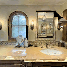
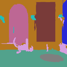
Matterport3D (MP3D) [1] is a large-scale dataset introduced in 2017, featuring over 10k images of 90 different building-scale indoor scenes. The dataset provides annotations with surface reconstructions, camera poses, color and depth images, as well as semantic segmentation images. For our project, we use a different version of this dataset which can be obtained through the Habitat Simulation environment described in Section 1.2. It is important to note that one of the major differences between this version of the dataset and the original one is that in the former, images have lower resolution and quality. As it can be observed in Figure 1, the images exhibit visual artifacts, making the task of 3D learning more challenging.

As such, this particular version of the dataset has been generally used for training Embodied agents in various multi-modal navigation tasks [2, 3, 4]. We explore this version of the dataset since we are interested in equipping Embodied agents with 3D learning and understanding skills within this simulation platform.

2.1.2: Simulation and Trajectories

In order to generate the data for training, validation and testing, we used the Vision-and-Language (VLN) dataset presented in [2]. This dataset consists of instructions provided in natural language that describe a particular path to follow in a MP3D indoor environment. These instructions correspond with a trajectory in the environment which can be obtained by using a Shortest-Path-Follower (SPF) from the start and goal locations associated with the instruction. For this project, we are not interested in the language instructions. Thus, we do not provide details on how this dataset has been used to train instruction-following agents. However, we leverage the visual trajectories associated to such instructions for creating our dataset.

The VLN dataset described above was designed for the Habitat [5] simulation platform. Thus, we use [5] to collect the data for training. Briefly, Habitat is a highly efficient and flexible platform intended for embodied research. It allows researchers to easily design and configure agents and sensors, as well as AI algorithms for a diverse set of navigation tasks [2, 3, 4].

Specifically, we use a SPF, as described above, to get the sensor information from the simulator based on the VLN dataset. We specifically, extract RGB, depth and color images for each trajectory, as well as, relative pose information. The SPF uses has an action space consisting of four possible actions: MOVE_FORWARD 0.25m, TURN_LEFT 15deg, TURN_RIGHT 15deg, and STOP. An example of a resulting trajectory is shown in Figure 1.

Table 1. shows statistical information about the dataset we obtained.

Table 1. Dataset statistics
Data Split Num. Environments Avg. Num. Trajectories per Environment Total Num. Trajectories Avg. Num. Steps per Trajectory Total Num. Steps per Trajectory
Train 33 65 2,169 55 119,976
Val 33 5 142 54 7,750
Test 11 55 613 54 33,412

2.2 Model

As mentioned before, we focus on learning the 3D structure of an indoor environment from video sequences. We follow prior work [6], which focuses on learning Structure-from-Motion (SfM) in outdoor environments. This model achieves the latter purely from training on unlabeled color images and through a view-synthesis objective function as their main supervisory signal.

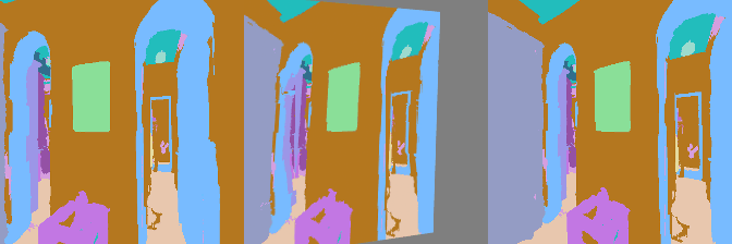
In our project, we explore if explicitly incorporating semantic information, in the form of masks, enables the model to better understand and learn to model the 3D structure of a given scene. Our model jointly trains two neural networks; one in charge of predicting depth from a single-view image represented both in RGB and in semantic labels, and the other in charge of predicting the pose transformaton between two images. To train the model, we also use a view-synthesis objective for both the color images and the segmentations and a multi-scale smoothness loss. Section 2.1 and Section 2.2 provide more details on the model implementation, and Section 2.3 dives into the details of the objective functions.

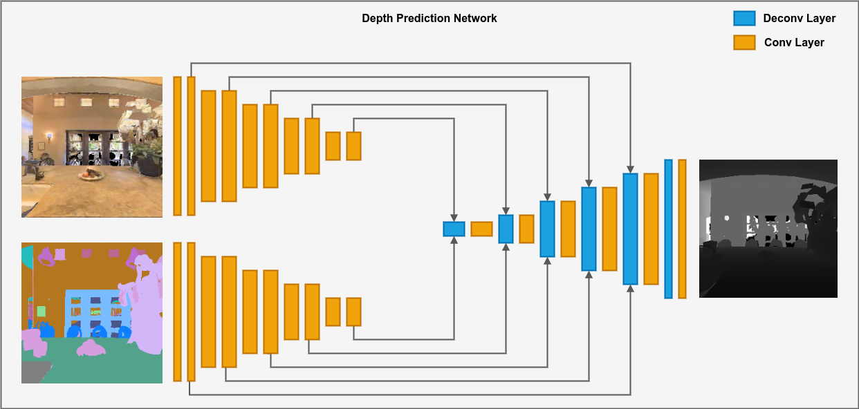
2.2.1. Depth Network

The first component of the model is the Depth Network, a CNN-based model which takes as input a target image represented in color information and semantic masks and outputs the corresponding depth information. As shown in Figure 2, the Depth Network is comprised by two encoders, one for each input modality, i.e., color and semantic masks, and one decoder which uses the concatenated embeddings of each of the encoders to predict the corresponding depth.
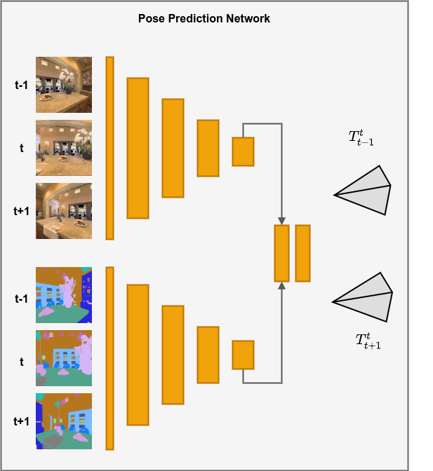
Figure 2. Depth Prediction Network

2.2.2. Pose Network

The second component of the model is the Pose Network, which is also a CNN-based network. This module takes as input a short sequence of N images also represented in color and semantic masks. Here, one of the images in the sequence is the target image It and all other images are the sources Is. The model then outputs the pose transformation between all source images and the target image. Like the Depth Network, the Pose Network is comprised by two encoders, one for each input modality. Then, the final embeddings of each encoder are concatenated together and used to predict the pose transformations between the images. The model is shown in Figure 3.

Figure 3. Pose Prediction Network

2.2.3: Objective Functions
2.2.3.1: View Synthesis

The main objective function in this project comes from a view synthesis task: given one input view of a scene, \(I_t\), the goal is to synthesize a new image of the scene from a different camera pose. In [6], the synthesis process is achieved by predicting both the depth information of a target viewpoint, \(D_t\), and the pose transformations between the target view, \(T_{t \rightarrow n}\), where \(n\) is the sub-script of the nearby view, \(I_n\). Here, the depth and pose information is learned through the CNN-based modules, which were explained in the previous sections.

The view-synthesis objective is given by the following equation: $$ L_{vs} = \sum_{n} \sum_{p} | I_t(p) - \hat{I}_n(p) | $$ where \(p\) is a pixel index, and \(\hat{I}_n\) is a nearby image warped into the target's coordinate frame. To warp the nearby image to the target frame, we can project \(p_t\), a homogeneous coordinate of a pixel in the target image onto the nearby image by following the equation below, $$ p_n \sim K \cdot T_{t \rightarrow n} \cdot D_t(p_t) \cdot K^{-1} \cdot p_t $$ where \(p_t\) represents the homogeneous coordinates of a pixel in the target image, \(K\) is the intrinsics matrix, \(D_t\) and \(T_{t \rightarrow n}\) are the predicted depth and pose, respectively.

Now, the coordinate from the previous equation correspond to continous values. To obtain the value \(I_n(p_n)\) to represent \(\hat{I}_s(p_t)\), we follow two interpolation methods: 1) bilinear interpolation for color images, which linearly interpolates the top-left, top-right, bottom-left and bottom-right pixel neighbors, and 2) nearest interpolation for the semantic masks, to preserve the original label values.

Thus, in summary, the view-synthesis objective is applied to both the color images and the semantic masks by warping the source image into the target frame using the predicted depth and poses, as well as the corresponding interpolation method.

2.2.3.2: Artifact Mask

Unlike [6], the scenes in our indoor environments are assumed to be static, i.e., there are no dynamic objects at any point in a given sequence. However, existing challenges with the dataset include 1) occluding objects and 2) visual artifacts at certain viewpoints resulting from the low quality reconstructions of the images.

To deal with this, the Pose Network is coupled with an Artifact Network which is trained to predict a pixel mask, \(E_n(p)\) that represents whether a pixel contributes to modeling the 3D structure of a given environment. This mask is used to weigh each pixel coordinate in the view-synthesis loss as, $$ L_{vs} = \sum_{n} \sum_{p} E_n(p) | I_t(p) - \hat{I}_n(p) $$ To avoid the network to predict an all-zeroes mask, the objective is coupled with a regularization term, \(L_{reg}(E_n)\).

2.2.3.3: Large Spatial Regions

The final objective function is used to explicitly allow to propagate gradients from large spatial regions in the image, as opposed to only considering the 4 local neighbors of the pixel, as explained in Section 2.3.1. To do this, depth maps are predicted at different scales and the \(L_1\) loss of their second-order gradients is minimized as in [6].

The final loss then becomes: $$ L = \sum_{l} L_{vs}^{l} + \lambda L_{ms}^{l} + \beta \sum_{n} L_{reg}(E^{l}_n)$$ here, \(l\) is the index of the image scale, \(L_{ms}\) is the multi-scale loss and \(\lambda\) and \(\beta\) are weighing hyper-parameters.


3. EXPERIMENTS

Our experiments were conducted in a server equipped with 4 GeForce RTX 2080 GPUs, each with 10GB of memory, Ubuntu 18.04, Pytorch 1.11 and CUD4 11.4. With this setup, each experiment took around 4-5 days to complete. For this reason, we were only able to define and train three main experiments without the possibility to run experiments for hyper-parameter search. Below, we list the conducted experiments and their corresponding hyper-parameters:

  1. RGB-only In this experiment we simply adapted the model introduced in [6] to work on our dataset.
  2. Artifact Mask In this experiment an artifact mask was generated in order to mask out occlusion pixels that were less relevant to the prediction of the next frame.
  3. RGB and Semantic Encoded In this experiment both RGB and semantic information is used. As explained in the Approach section, we extend the model introduced in [6] to generate semantic embedings and used them as context for predicting depth.

Table 2. Hyper-Parameter setup. VS, SVS, MS and MR refer to the weights used view sythesis, semantic view synthesis, multi-scale and mask regularization losses, respectively.
Experiment Epochs Learning Rate Optimizer Batch Size VS SVS MS MR
1 115 0.0002 Adam 8 1 N/A 0.1 N/A
2 115 0.0002 Adam 8 1 N/A 0.1 0.2
3 115 0.0002 Adam 8 1 1 0.1 N/A

4. RESULTS

In this section, we compare the results obtained on each of our proposed experiments. Because the approach is modular, both the depth network and pose network can be independently assessed. As such, we designed both qualitative and quantitative experiments for these modules. In the paragraphs that follow, we explain each experiment in more detail and show according results for each experiment.

4.1 Training curves

Before diving into the qualitative results, we briefly show and discuss, the trainining curves for each experiment in Figure 4. First, we can observe that Experiment 1 had an underfitting behavior: it converged to a high loss and its validation curve had the highest loss values out of all three experiments. Then, we can see that Experiment 2 exhibits the lowest loss values in both curves which is expected since this experiment makes use of the Artifact Mask. However, the model barely improves from its initial loss value. Finally, Experiment 3 has the highest loss value during training due to the additional semantic loss. Nonetheless, the validation loss achieves lower loss values as compared to Experiment 1.

Figure 4. Training (top) and validation (bottom) curves.


4.2 Qualitative Results
4.2.1 Depth Network

For this qualitative experiment, we simply ran depth inference on a set of trajectories from the test set. It should be noted that, in contrast to the validation set, the environments in the test set were never seen by the networks. The environments in the validation set are the same as those found in the training set. The only difference are the trajectories.

In Figure 5 we show depth predictions for Experiment 1 (left-most) Eperiment 2 (center) and Experiment 3 (right-most). First, analyzing the depth results from Experiment 1 (1st and 2nd columns), we can observe that only using RGB images on this dataset, the model markedly underfitted which is consistent with the curves shown in Figure 4. Here, regardless of the environment and trajectory, the model always predicts very similar results that look like two bright vertical rectangles to the left and right and a darker rectangle to the center. The model also does not seem to understand depth, as it tends to predict darker spots on the bottom center, whereas it should be the opposite since in these visualizations darker means further away.

In the second experiment (3rd and 4th columns), which studies the effect of the Artifact Mask, it seems that the model better understands depth. It tends to predict ceilings to be further away (a darker color) and floors at the bottom-center to be closer (a lighter color). Nonetheless, depth predictions are generally more blurry than the other two experiments.

Finally, in the third experiment (5th and 6th columns) we observe that with semantic information taken into account, the predicted depth better captures the structure of the environments. For example, features like door frames, stairs, etc., appear much clearer. However, every few frames, the model predicts highly blurry images that follow the same diagonal gradient pattern. There is a bright patch at the top-left corner and a dark patch at the bottom-right corner. We posit that this strange behavior may be due to several reasons, for instance:

  1. The model was not explicitly trained to handle occlusions or visual artifacts.
  2. There are repetitive patterns in the semantic masks.
  3. The shortest-path-follower algorithm we used to obtain the data tends to navigate close to walls and obstacles. For example, if the agent is navigating very close to an object on the wall, i.e. a bookcase, it would show up with some features in RGB. However, this same bookcase would show up as a huge featureless colored blob in the semantic mask. We theorize that the gradients that are seen here result from the sharp cutoff between this semantic featureless blob and the rest of the scene.

Figure 4. Depth predictions. Experiment 1 (1st and 2nd cols), Experiment 2 (3rd and 4th cols) and Experiment 3 (5th and 6th cols).


4.2.2 Pose Network

For this evaluation, we ran pose inference on the same set of trajectories as we did with the depth network. Specifically, we provide the network with a viewpoint at some time step \(t\) and another viewpoint at time step \(t+1\). Then, we predict the pose transformation between them using either the ground truth depth or the predicted depth. Finally, we warp the image at time-step \(t+1\) to the coordinate frame of the image at time-step \(t\) and display the corresponding result.

We show the resulting warps for Experiment 1 in Figure 6. In each row, the left-most image sequence always show the image at time step \(t\), the right-most show the image a time step \(t+1\), and the ones at the center are the warps. Here, we used the corresponding ground truth depth. Figure 7 shows one example comparing the resulting warps when using ground truth depth (top) vs predicted depth (bottom).

Figure 6. Experiment 1 warps. The left-most sequence corresponds to images at time-step \(t\). The right-most sequence corresponds to images a time-step \(t+1\). The sequence at the center corresponds to the warped images from \(t+1\) to \(t\).

As you can see below in Figure 7, pose warping based on ground truth and predicted depth both give somewhat similar results. However, with predicted depth, the results tend to be slightly more bent and crooked. This is the same case for all three experiments.

Figure 7. Experiment 1 warps comparing the use of ground truth depth (top) vs predicted depth (bottom).


The resulting warps for Experiment 2 are shown in Figure 8. Since this experiment considers the Artifact Mask, we also display the corresponding mask for each time-step. Like the previous experiment, we also compare the results when using ground truth depth vs predicted depth in Figure 9.

Analyzing the predicted masks, we conclude that this method did not achieve what we intended: the predicted masks do not predict occluding objects nor visual artificats. In fact, in several cases, the masks predict large parts of the image. This may explain why the loss for the artifact mask during training and validation was the lowest, and why it did not improve significantly throughout the entire process. As you can see in the third column, there is significant warping in the outputs generated using the artifact mask.

Figure 8. Warp predictions for experiment 2.

Figure 9. Experiment 2 warps comparing the use of ground truth depth (top) vs predicted depth (bottom).


The resulting warps for Experiment 3 are shown in Figure 10. Since this experiment leverages semantic information, we also display the corresponding warps for the semantic masks. Finally, Figure 11 compares the results when using ground truth depth vs predicted depth.

As you can see, there is pretty significant warping in some of the generated outputs. We acknowledge that, this could be due to the relatively small number of epochs we were able to train the model and that we were also unable to run hyper-parameter search experiments. We expect that these results should improve as more experiments are carried and the effect of each hyper-parameter is more throughly understood.

Figure 10. Warp predictions for experiment 3.

Similar to Fig. 7, Fig. 11 compares the results of warping based on ground truth and based on predictions of the next frame. Again, warping based on ground truth produces slightly better results than those that were based on predictions.

Figure 11. Experiment 2 warps comparing the use of ground truth depth (top) vs predicted depth (bottom).


4.3 Quantitative Results
4.3.1 Depth Network

In Table 3 we compare the ground truth depth and the predicted depth for each experiment and report three error metrics also reported in [6]:

  1. Abs rel: is the absolute error relative to the ground truth values.
  2. Sq rel: is the squared error relative to the ground truth values.
  3. RMSE: is the root mean squared error of the difference between the ground truth and the prediction.

These results show that Experiment 1 acheived significantly lower error as compared to the other two experiments. Nonetheless, from visual inspection in Section 4.2.1 we observed that Experiment 1 underfit to the training process. The reported errors for the remaining two experiments are similar. As we discussed before, these experiments showed various limitations: in Experiment 2 the predicted depths are very blurry, and in Experiment 3 the repeated diagonal pattern may have drastically affected the predictions.

Table 3. Depth Error Metrics
Experiment Abs Rel Sq Rel RMSE
1 0.706 0.113 0.146
2 2.091 1.841 0.325
3 2.300 4.900 0.451

4.3.2 Pose Network

In Table 4 we compare the ground truth poses obtained using the Habitat simulator and the predicted pose information for each experiment and report three error metrics also reported in [6]:

  1. ATE: absolute trajectory error
  2. RE: rotation error

These results show that Experiment 2 acheived slighlty lower pose error compared to the other two experiments. Nonetheless, from visual inspection in Section 4.2.2 it is difficult to assess whether this model's predicted poses are in fact "better" since the warps are more marked for the latter two experiments.

Table 4. Pose Error Metrics
Experiment ATE RE
1 0.0203 0.2006
2 0.0164 0.1429
3 0.0219 0.1554

DISCUSSION

Through the 3 experiments conducted, we discovered the following:

  1. RGB-only experimental cases tended to underfit the dataset with high training and validation loss. Resulting in the visualizations which tended to all look the same, regardless of what environment they were generated from.
  2. The RGB and Artifact mask experimental case tended to do better than RGB-only in understanding depth. For instance, darker regions were more often predicted at the ceilings or at the center of the image (representing objects that were further away) and viceversa. Nonetheless, the predicted depths tended to be more blurry, and the warps were significantly more marked.
  3. The RGB and semantic mask experimental case gave very unexpected diagonal gradient-like results. We believe this to be the result of the shortest path follower algorithm sticking the corners of the environments. Due to this, it is more likely to encounter large featureless semantic mask blobs that take up most of its FOV, thus generating a diagonal gradient across the screen.
  4. The artifact mask ended up masking out most of the relevant parts of a scene. This experiment did not work as expected, and therefore produced extremely warped outputs.

Despite these interesting quirks and all the challenges we faced, e,g., having a low quality dataset, to having limited resources for training more experiments and better analyzing the effect of our hyper-parameters and loss functions, etc, we got interesting results on the indoor scenes and trajectories given by the MatterPort3D dataset. We believe that the model would be even more accurate at portraying these indoor trajectories if they were given more time and resources for training more experiments to better understand the hyper-parameters.

Some things that we can try going forward include:

  1. 3D point loss: 3D spatial information is considered for this kind of loss. The depth map for the specified target frame can be used to grab 3D coordinates for a specific pixel in the target frame. In a similar method, the 3D coordinates for the source pixel associated with that specific target pixel can be obtained by applying a transformation matrix to the depth maps. After these two have been obtained, 3D loss can be calculated as the difference between the transformed source and target pixel. This loss would be more appropriate for analyzing 3D structures and better understanding occluding objects.
  2. Improve multi-scale loss: As pointed out in [8], the current multi-scale loss has a tendency for creating "holes" in large low texture regions in lower scale depth maps. One improvement proposed in [8] consists of up-sampling the lower scale depth maps to the input scale and then compute the multi-scale photometric error. They showed this to be an effective idea that allows them to constrain the depth maps at all scales to work on the same objective: reconstruct the input-resolution image.
  3. Improve generated trajectories: Address the issue of the shortest-path-follower that navigates close to obstacles as opposed to centered to the path it follows. For instance, when we walk in a hallway, we generally walk centered to it, as opposed to following the wall edges. This would allow us to get better viewpoints that are less occluded by large objects like walls.

REFERENCES

  1. Matterport3D: Learning from RGB-D Data in Indoor Environments [link]
  2. Beyond the Nav-Graph: Vision-and-Language Navigation in Continuous Environments [link]
  3. SoundSpaces: Audio-Visual Navigation in 3D Environments [link]
  4. DD-PPO: Learning Near-Perfect PointGoal Navigators from 2.5 Billion Frames [link]
  5. Habitat: A Platform for Embodied AI Research [link]
  6. Unsupervised Learning of Depth and Ego-Motion from Video [link]
  7. KITTI Dataset [link]
  8. Semantics Driven Unsupervised Learning for Monocular Depth and Ego Motion Estimation [link]
  9. Digging into self-supervised monocular depth estimation [link]