Return to the lecture notes index
Lecture 10 (Tuesday, February 17, 2009)
Failure and Storage
Last class, we discusses error-correction and error detection codes and
their applicability to data communication. Today, we're going to talk
a little bit about reliability and storage.
In discussing EDCs and ECCs, as used in communications, we said that ECCs
are very rarely used. Instead, the most common approach is simply to
resend the data, if appropriate. The only exception we carved was in
intrinsicly noisy, but high-bandwidth channels, such as satellites.
In these cases, ECCs make sense, because they enable us to make use of
a media that, otherwise, might be too noisy to use.
But, when it comes to storage systems, such as disks, ECCs are an
intinsic part of the system by design. If we lose the data, we can't
just go back to the well. There is no where to go.
And, as it turns out, modern disks are technological marvels obtaining
a tremendous information density at tremendous speeds by pushing the media
and the technology right to its tolerances. Getting a bit wrong here
or there isn't tremendously rare -- disks regularly use ECCs to deliver
data. ECC logic is built directly into the controllers and is applied
with every read and write.
It is worth noting that, in addition to protecting against read/write
problems, good storage systems protect against power failure, cabling
failure, human error, &c.
Failure and Scale
In the real-world many devices experience a "bath tub" like failure
model. The highest rate of failure is dead-on-arrival units and those
that failure during a burn-in period. So, we start out with a high
failure rate that quickly drops off to a low, stable rate of failure,
where it remains for years. But, eventually, as the devices age, failures
cease being rare. Once the failure rate increases, it seems to hang out
in this final phase of aging, a steadily, but slowly increasing failure
rate, until the last of the units die.
But, for the purpose of this discussion, let's ignore this common, real-world
failure model and do some really broken, but simple, math. Suppose the
mean time between failures (MTBF) of the average disk is 50,000 hours --
about 6 years. Now imagine that we have 100 disks in service. We can expect
a failure every 500 hours: 1 failure/50,000 hours/disk * 100 disks =
1 failure/100 hours. So, we now expect a failure every few weeks.
Even if this is over simplified, it does highlight the fact that as
the quantity scales up -- so do failures. Beyond a certain point, failure
is the steady-state, not the exception. Any system that operates beyond
a certain scale must be designed to work each and every day with failed
components. I honestly doubt that the Googles of the world bother to
replace things as they break. I suspect that they just let them fail
and replace them only when it is time for an upgrade or a whole rack of
components fail or the sprinkler system accidentally gets turned on, I
dunno'.
So, today's lecture is a case study in managing failure -- RAID arrays.
They were once an extravagance in high-end systems, but are now the
backbone of performance and reliablity in even modest configurations.
Let's take a look at how they use redundancy to achieve reliability
and performance, despite scale.
Redundant Arrays of Independent (formerly, Inexpensive) Disks (RAID)
The goal of most RAID systems is to improve the performance of storage
systems. The idea is that, instead of building/buying more expensive disks,
we can use arrays of commodity disks organized together to achieve
lower latencies and high bandwidths.
But, as we scale up the number of disks required to store our data, unless
we do something special, we'll also scale up the liklihood of us losing
our data due to failure. So, what we are actually going to discuss is
how to organize disks to achive better performance (lower latency and/or
higher bandwidth) as well as greater reliability (fail-soft or fail-safe).
RAID - Striping
RAID systems can obtain increased bandwidth by distributing data across
several disks using a technique is called striping. The result of
this technique is that the bandwidth is not limited by a single drive's
bandwidth, but is instead the sum of the bandwidth of several drives.
When we think about I/O with RAIDs, we don't think in terms of sectors or
blocks. Instead we think about stripes A stripe is an abstraction
that represents the fundamental unit of data that can be written
simultaneously across several disks. The amount of data that can be stored
in a stripe is called the stripe width. A portion of the stripe is
stored on each of several disks. This portion is caled the stripe unit.
The size of the stripe unit is the number of bytes of a stripe that are
stored on a particular disk.
If the stripe width is S bytes and we have N disks available to store user
data, the strip unit is S/N bytes. For example, if a RAID has 5 disks
available to store user data, and the stripe width is 100K, each stripe
unit is (100K/5) 20K.
If the application or OS I/O buffer cache reads an entire stripe at a time,
the array controller can perform parallel accesses to all N disks. The
bandwidth as viewed by the user is not the bandwidth of each individual
disk, but is instead the aggregate bandwidth accross all disks.
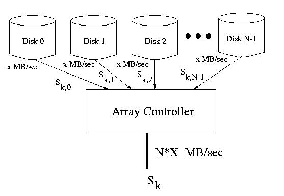
Figure: An entire stripe delivered at once from several disks at N * X MB/sec
If several requests are made concurrently, it may be possible to service
all or some of them in parallel. This is because requests for data living
in strip units on different disks may be performed in parallel. In this way
the array can service multiple requests at the same time. Of course, if the
requests live in stripe units on the same disk, the requests must still be
serialized.
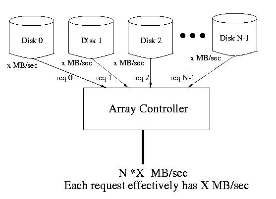
Figure: N requests serviced at once from N different disks each at X MB/sec
If we hold constant the number of disks available for user data, we can
tune the performance of the array by varying the stripe unit size:
-
If the goal is to increase throughput, a single request must be
handled in parallel across several disks. To achive this the stripe unit size
must be small with respect to the size of the request, ensuring that
requests requires multiple stripe units. The stripe unit can then be
accessed in parallel on different disks. This parallelization improves
throughput. This is often useful, for example, on servers where the
requested data is probably randomly distributed across the several disks.
This implies that there is a good liklihood that many of the requests can
be parallelized.
-
If the goal is to decrease latency, each request should be confined
to a single disk within the array. This leaves the other disks available
to service other requests in parallel, thereby decreasing their waiting time
and consequently the observed latency. To achive this, the stripe unit
size should be made large with respect to the size of the request.
If the request is confined to a single stripe unit, the other disks in
the array will be available to service other requests concurrently.
Many commercially available arrays allow the administrator to select from
several available stripe unit sizes when the disk is first initialized.
Other arrays are not configurable, so this becomes a purchase-time
consideration.
Improving Reliability
In order to improve the reliability of these arrays, we'll make use
of redundancy. In particular, we'll either mirror a copy of the
data directly to a redundant disk, or we'll add parity or other
error-correction codes to the system that enable us to recover from
disk failure.
It is important that, at this point, we are discussing parity across
disks that enables us to recover from the complete failure of an entire
disk, rather than the incormporation of ECCs into a single disk, which
enable the recovery of small amounts of corrupted data on an otherwise
functioning disk.
RAID Approaches
There are many approaches to achieving the redundancy required in arrays.
Although there are other classifications, most commercial RAIDS fall into
categories known as levels: RAID level 1 - RAID level 6.
There are several metrics that can be used to evaluate alternatives:
- How much space is wasted by redundancy?
- What is the likelihood of hot spots during heavy loads?
(Hot spots are parts of the disk that are accessed sufficiently
more frequently that they cause a bottleck.)
- How much does performance degrade when a disk fails or during
a repair?
RAID Level 1
Raid level 1 is also known as Mirroring. Disks within the
array exist in pairs -- a data disk and a corresponding backup
disk. Blocks can be read from either disk in the pair, but in the normal
case, data is always written to both disks. Depending on the assumptions
about the types of failure, the writes to the data and backup disks may
or may not be performed in parallel.
In the event of a failure, data is read and written to and from the
working disk. After the defective disk is replaced, the data can be
reconstructed from its twin.
It is also possible to locate the mirror disks miles and miles apart.
This insulates the data from a location-indiuced failure like an
earthquake, flood, or fire.
| Data Disk 1 |
Backup Disk 1 |
Data Disk 2 |
Backup Disk 2 |
... |
Data Disk 3 |
Backup Disk 3 |
RAID Levels 2 & 3
RAID levels 2 & 3 use bit-interleaved error-correction schemes.
This means that the redundant information required to correct errors
is calculated on a bit-wise basis from corresponding bits across the
several disks. This means that all heads must always move in lock-step.
RAID Level 2 uses an ECC similar to that used in many silicon-based memories.
Often times, a Hamming code is used -- this requires Log (N) disks be
used for error correction.
RAID level 3 uses a simple parity bit. Although simple parity can not
in general be used as an error correcting code, just as an error detection
code, this isn't the case with disks. Most often we can determine which
disk has failed. Provided no other errors occur, the parity bits can be used
to determine the value of each bit on the failed disk. The good
news is that only one parity disk is required, and this expense is amortized
over all data disks.
RAID level 2 is rarely implemented because of the number of disks required
for redundancy. ECCs are unnecessary given the reasonably high level of
reliability of most disks.
Although RAID level 3 doesn't suffer this difficulty, it is also rarely
implemented. Since all of the heads must move in lock-step, this type
of array can't really support concurrency.
RAID Level 4
Unlike RAID levels 2 & 3, RAID Level 4 is designed to allow concurrent
accesses to the disks within the array. it maintains the small wastage
of RAID level 3.
This is achived by using block-interleaved parity. One disk contains
only parity blocks. Each parity block contains the parity information
for corresponding blocks on the other disks. Each time a write is
performed, the corresponding parity block is updated based on the
old parity, the old data, and the new data.
The parity bit is the XOR of corresponding bits across all disks.
Consider the example below:
Since the parity disk must be accessed every time a write is performed
to any other disk, it becomes a hots spot.
| Disk 0 |
Disk 1 |
Disk 2 |
Parity Disk |
| D0,0 |
D0,1 |
D0,2 |
P0 |
| D1,0 |
D1,1 |
D1,2 |
P1 |
| D2,0 |
D2,1 |
D2,2 |
P2 |
| D3,0 |
D3,1 |
D3,2 |
P3 |
P0 = D0,0 XOR D0,1 XOR
D0,1
Although it might initially seem that every disk must be accessed each
time any disk is written, this is not the case. Given the old parity,
the old data value, and the new data value, we can computer the new
parity without reading any other disk.
Consider a write to D0,2, the new parity can be computed as
follows:
P0-new = (D0,2-old XOR D0,2-new)
XOR P0-old
Normal read operations require access only to one disk. Normal write
operations require access to the target disk and to the parity disk.
Once any data disk fails, read and write operations require access to
all disks. The corresponding parity bit and data bits are XOR'd to calculate
the missing data bit.
RAID Level 5
RAID level 5 operates exaclty as does RAID level 4, expect that the
parity block are distributed among the disks. This distributs the
parity update traffic among the disks, alleviating the hot spot of
the single parity disk. Typically the parity blocks are placed
round-robin in a rotated fashion on the disks. This is known as
rotated parity
| Disk 0 |
Disk 1 |
Disk 2 |
Disk 3 |
| D0,0 |
D0,1 |
D0,2 |
P0 |
| D1,0 |
D1,1 |
P1 |
D1,3 |
| D2,0 |
P2 |
D2,2 |
D2,3 |
| P3 |
D3,1 |
D3,2 |
D3,3 |
P0 = D0,0 XOR D0,1 XOR
D0,1
P3 = D3,1 XOR D3,2 XOR
D3,3
Normal read operations require access only to one disk. Normal write
operations require access to the target disk and to the disk hold
the parity for that data block.
Once any data disk fails, read and write operations require access to
all disks. The corresponding parity bit and other data bits are XOR'd
to calculate the missing data bit.
RAID 6
RAID 6 is essentially identical to RAID 5, except that it incorporates
two different parity blocks. This enables it to function through not only
one, but two, disk failures -- for example a disk failure during the
replacement and reconstruction from a prior disk failure.
As disks become larger and recovery times increase, the window of vulnerability
for a second failure also increases. RAID 6 guards against this and is
increasingly being seen as essential in high-reliability systems.
Hamming Distance and RAID Levels 3-6?
If we need a Hamming distance of (2D + 1) to detect a bit bit error, how can
we get away with only one parity disk -- don't we need Log 2 N,
as above?
Actually no. The big difference between disks and memory or a network is that
we can ususally which disk has failed. Disk failures are usually catrastrophic
and not transient. If we know which disk has failed, which is usually
easy to figure out, we can correct a 1-bit error, given simple parity. We
just set that bit to whatever it needs to be for the parity bit to be correct.