Return to the Lecture Notes Index
15-200 Lecture 29 (Monday, November 14, 2005)
Dijkstra's Algorithm: Shortest Path Algorithm for Weighted Graphs
One common use of graphs is to find the shortest path from one place to
another. You may have at some point used an online program to find driving
directions, and you likely had to specify if you wanted the shortest
route/fastest route. This involves finding the shortest path in a weighted
graph.
The general algorithm to solve the shortest path problem is known as
Dijkstra's Algorithm. With Dijkstra's algorithm, we proceed in stages.
At each stage, we can calculate with certainty the shortest path to a new vertex.
We then keep finding the shortest path to new vertices, until we have found the
shortest path to the vertex that we want.
As we go, we'll keep track of the current shortest known path to each vertex in the graph.
We'll also keep track of wether or not we know for certain that this path is the shortest
possible path. We can figure out that a path is the shortest possible if we've already seen
that any other path through the graph must be at least that length.
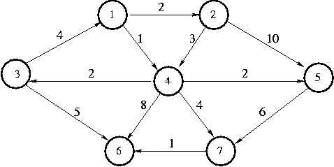
For example, suppose we have the following graph:

This graph is a directed graph, but it could just as easily be
undirected.
Let's call the starting vertex s vertex 1. Just a reminder
before we begin: the point of a shortest path algorithm is to find the
shortest path to s from each of the other vertices in the graph.
The first vertex we select is 1, with a path of length 0. We mark
vertex 1 as known.
|
| Known
| Path
| Length
|
| 1
| Y
| 1
| 0
|
| 2
| -
| -
| INF
|
| 3
| -
| -
| INF
|
| 4
| -
| -
| INF
|
| 5
| -
| -
| INF
|
| 6
| -
| -
| INF
|
| 7
| -
| -
| INF
|
The vertices adjacent to 1 are 2 and 4.
We adjust their fields.
|
| Known
| Path
| Length
|
| 1
| Y
| 1
| 0
|
| 2
| -
| 1
| 2
|
| 3
| -
| -
| INF
|
| 4
| -
| 1
| 1
|
| 5
| -
| -
| INF
|
| 6
| -
| -
| INF
|
| 7
| -
| -
| INF
|
Next we select vertex 4 and mark it known. Vertices 3,
5, 6, and 7 are adjacent to 4, and we can
improve each of their Length fields, so we do.
|
| Known
| Path
| Length
|
| 1
| Y
| 1
| 0
|
| 2
| -
| 1
| 2
|
| 3
| -
| 4
| 3
|
| 4
| Y
| 1
| 1
|
| 5
| -
| 4
| 3
|
| 6
| -
| 4
| 9
|
| 7
| -
| 4
| 5
|
Next we select vertex 2 and mark it known. Vertex 4 is
adjacent but already known, so we don't need to do anything to it.
Vertex 5 is adjacent but not adjusted, because the cost of
going through vertex 2 is 2 + 10 = 12 and a path of length 3 is
already known.
|
| Known
| Path
| Length
|
| 1
| Y
| 1
| 0
|
| 2
| Y
| 1
| 2
|
| 3
| -
| 4
| 3
|
| 4
| Y
| 1
| 1
|
| 5
| -
| 4
| 3
|
| 6
| -
| 4
| 9
|
| 7
| -
| 4
| 5
|
The next vertex we select is 5 and mark it known at cost 3.
Vertex 7 is the only adjacent vertex, but we don't
adjust it, because 3 + 6 > 5. Then we select vertex 3, and adjust the
length for vertex 6 is down to 3 + 5 = 8.
|
| Known
| Path
| Length
|
| 1
| Y
| 1
| 0
|
| 2
| Y
| 1
| 2
|
| 3
| Y
| 4
| 3
|
| 4
| Y
| 1
| 1
|
| 5
| Y
| 4
| 3
|
| 6
| -
| 3
| 8
|
| 7
| -
| 4
| 5
|
Next we select vertex 7 and mark it known. We adjust vertex 6
down to 5 + 1 = 6.
|
| Known
| Path
| Length
|
| 1
| Y
| 1
| 0
|
| 2
| Y
| 1
| 2
|
| 3
| Y
| 4
| 3
|
| 4
| Y
| 1
| 1
|
| 5
| Y
| 4
| 3
|
| 6
| -
| 7
| 6
|
| 7
| Y
| 4
| 5
|
Finally, we select vertex 6 and make it known. Here's the final table.
|
| Known
| Path
| Length
|
| 1
| Y
| 1
| 0
|
| 2
| Y
| 1
| 2
|
| 3
| Y
| 4
| 3
|
| 4
| Y
| 1
| 1
|
| 5
| Y
| 4
| 3
|
| 6
| Y
| 7
| 6
|
| 7
| Y
| 4
| 5
|
Now if we need to know how far away a vertex is from vertex 1,
we can look it up in the table. We can also find the best route, for
example, from the starting city (the one we selected as the route) to
any other city (any other node). We just use the Path field to find
the destinations predecessor, then use that node's path field to find
its predecessor, and so on.
Shortest Path Algorithm for Unweighted Graphs
Unweighted graphs are a special case of weighted graphs. They can
be addressed using Dijkstra's algorithm, as above -- just assume
that all of the edges weigh the same thing, such as 1. Or, we
can actually take a little bit of a shortcut.
For unweighted graphs, we don't actually need the "known" column
of the table. This is because as soon as we discover a path to a
vertex, we have discovered the best path -- there is no way we
can find a better path. As a result, the verticies become
"known" as soon as we find the first way to get there. We might
subsequently find an equally good way -- but never a better way.
Let's think about the situation in Dijkstra's Algorithm that resulted
in the discovery of a "better" path to a vertex that was already
reachable. This situation occured, if a path with more "hops"
was shorter than a path with fewer "hops". In other words, Dijkstra's
algorithm reaches nodes in the same order as a breadth-first search
-- reaching all nodes one hop from the start, then those two hops from
the start, then those three hops from the start, and so on.
But, since not all of the hops are of the same length, one hop
might be really long, for example it might have a cost of 100.
But, another path between the same nodes, might involve three hops,
of lengths, 10, 20, and 30. It is cheaper to go the three hops
10+20+30=60 than the single hop of 100. Yet, the hop of 100 is
the path that is discovered first. As a result, we need to
check subsequent paths that pass through more verticies, until
we are sure that we can't find a better path, at which time,
we finally mark the node (and the path to it) as known.
Since, in an unweighted graph, all of the edges are modeled as
having the same weight, it is impossible for this situation
to occur. Two hops will always be longer than three hops, &c.
Since the algorithm is proceeding in a depth-first fashion,
we find things that are one hop away before things that are two
hops away, before things that are three hops away, and so on.
As a result, in an unweighted graph, as soon as we find a node,
it is known -- there can be no better way of finding it.
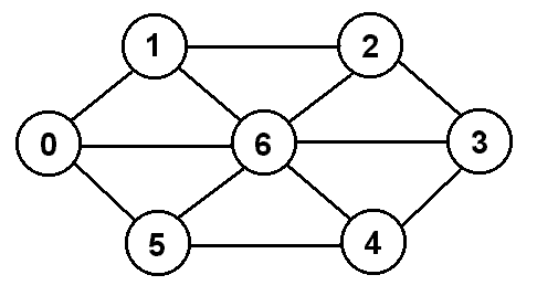
Let's consider an example for the graph shown below.

We would build a table as follows:
|
| Known
| Path
| Length
|
| 0
| -
| -
| INF
|
| 1
| -
| -
| INF
|
| 2
| -
| -
| INF
|
| 3
| -
| -
| INF
|
| 4
| -
| -
| INF
|
| 5
| -
| -
| INF
|
| 6
| -
| -
| INF
|
In the table, the index on the left represents the vertex we are going to
(for convenience, we will assume that we are starting at vertex 0).
This time, we will ignore the Known field, since it is only necessary
if the edges are weighted. The Path field tells us which vertex precedes
us in the path. The Length field is the length of the path from the
starting vertex to that vertex, which we initialize to INFinity under the
assumption that there is no path unless we find one, in which case the length
will be less than infinity.
We begin by indicating that 0 can reach itself with a path of length 0.
This is better than infinity, so we replace INF with 0 in the Length column,
and we also place a 0 in the Path column. Now we look at 0's
neighbors. All three of 0's neighbors 1, 5,
and 6 can be reached from 0 with a path of length 1
(1 + the length of the path to 0, which is 0), and for all
three of them this is better, so we update their Path and Length fields,
and then enqueue them, because we will have to look at their neighbors next.
We dequeue 1, and look at its neighbors 0, 2,
and 6. The path through vertex 1 to each of those vertices
would have a length of 2 (1 + the length of the path to 1, which is 1).
For 0 and 6, this is worse than what is already in their Length
field, so we will do nothing for them. For 2, the path of length 2 is
better than infinity, so we will put 2 in its Length field and 1 in
its Path field, since it came from 1, and then we will enqueue so
we can eventually look at its neighbors if necessary.
We dequeue the 5 and look at its neighbors 0, 4, and
6. The path through vertex 5 to each of those vertices would
have a length of 2 (1 + the length of the path to 5, which is 1).
For 0 and 6, this is worse than what is already in their
Length field, so we will do nothing for them. For 4, the path of
length 2 is better than infinity, so we will put 2 in its Length field and
5 in its Path field, since it came from 5, and then we will
enqueue it so we can eventually look at its neighbors if necessary.
Next we dequeue the 6, which shares an edge with each of the other six
vertices. The path through 6 to any of these vertices would have a
length of 2, but only vertex 3 currently has a higher Length
(infinity), so we will update 3's fields and enqueue it.
Of the remaining items in the queue, the path through them to their neighbors
will all have a length of 3, since they all have a length of 2, which will be
worse than the values that are already in the Length fields of all the
vertices, so we will not make any more changes to the table. The result is
the following table:
|
| Known
| Path
| Length
|
| 0
| -
| 0
| 0
|
| 1
| -
| 0
| 1
|
| 2
| -
| 1
| 2
|
| 3
| -
| 6
| 2
|
| 4
| -
| 5
| 2
|
| 5
| -
| 0
| 1
|
| 6
| -
| 0
| 1
|
Now if we need to know how far away a vertex is from vertex 0, we can
look it up in the table, just as before. And, just as before, we can use the
path field to discover the rout from the starting node to any vertex.
Prim's Algorithm
Next, we talked about a very similar algorithm. In fact, the actual algorithm is
pretty much exactly the same as Dijkstra's algorithm. The only difference is in
the "cost function".
In Dijksta's algorithm, we kept track of the current distance from the starting point.
This distance was cumulative, meaning it was the total distance from the start to the
current vertex. For Prim's algorithm, instead of keeping track of the cumulative distance,
we keep track of just the distance between the two consecutive vertices. Also, in Prim's
algorithm, we don't have a specific vertex that we are looking for. We continue the algorithm
until all paths have been exhausted. At this point, instead of having a shortest path,
the result will be a minimum spanning tree!
Imagine finding the minimum amount of sidewalk needed to get to every
point of interest from the entrance of a park. Now think of the park
entrance as the root of your minimum spanning tree. This will help you as
you apply Prim's Algorithm.
Like Dijktra's alogirthm, Prim's grows the tree in successive stages. You start by choosing one vertex
to be the root v, and add an edge (piece of sidewalk), and thus an
associated vertex (a point of interest in the park), to the tree. At each
stage, you add a vertex to the tree by choosing the vertex u such
that the cost of getting from v to u is the smallest possible
cost (in the case of the park, the cost is distance). At each stage,
you say, "Where can I get from here?" and go down the shortest road possible
from where you are.
Applying this algorithm until all vertices of the given graph are in the tree
creates a minimum spanning tree of that graph.
Prim's finds the minimum spanning tree of the entire graph from s, so we
use the Length field to record the cost of getting from a vertex v to
its parent in the minimum spanning tree we're making.
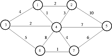
Suppose we have the following graph:

We would build a table as follows:
|
| Known
| Path
| Length
|
| 1
| -
| -
| INF
|
| 2
| -
| -
| INF
|
| 3
| -
| -
| INF
|
| 4
| -
| -
| INF
|
| 5
| -
| -
| INF
|
| 6
| -
| -
| INF
|
| 7
| -
| -
| INF
|
Selecting vertex 1 and making it the root of our tree, we update its
neighbors,
1, 2, 3, and 4. Vertex 1's cheapest place in the tree is known.
|
| Known
| Path
| Length
|
| 1
| Y
| 1
| 0
|
| 2
| -
| 1
| 2
|
| 3
| -
| 1
| 4
|
| 4
| -
| 1
| 1
|
| 5
| -
| -
| INF
|
| 6
| -
| -
| INF
|
| 7
| -
| -
| INF
|
Next we select vertex 4 (one of the neighbors of vertex 1). It's
cheapest place in the tree is now known. Every vertex in the graph is
adjacent to 4.
Vertex 1 is known (meaning that its in its optimal place in the tree),
so we don't examine it. We don't change vertex 2, because its Length is
2, and the edge cost from 4 to 2 is 3. We update the rest.
|
| Known
| Path
| Length
|
| 1
| Y
| 1
| 0
|
| 2
| -
| 1
| 2
|
| 3
| -
| 4
| 2
|
| 4
| Y
| 1
| 1
|
| 5
| -
| 4
| 7
|
| 6
| -
| 4
| 8
|
| 7
| -
| 4
| 4
|
Next we select vertex 2 (another neighbor of 1) and make it
known. We can't improve our tree in any way by going through vertex 2.
We select vertex 3 (the last neighbor of 1) and make it known.
The path from 3 to 6 is cheaper than the path from 4
to 6, so we update 6's fields.
2 and 3's cheapest places in the tree are now known.
|
| Known
| Path
| Length
|
| 1
| Y
| 1
| 0
|
| 2
| Y
| 1
| 2
|
| 3
| Y
| 4
| 2
|
| 4
| Y
| 1
| 1
|
| 5
| -
| 4
| 7
|
| 6
| -
| 3
| 5
|
| 7
| -
| 4
| 4
|
Next we select vertex 7 (neighbor of 4, the first chosen neighbor
of 1). Its cheapest place in the tree is now known. Now we can adjust
vertices 5 and 6. Selecting 5 and 6 doesn't
provide any cheaper paths. After 5 and 6 are selected, the
Prim's algorithm terminates.
|
| Known
| Path
| Length
|
| 1
| Y
| 1
| 0
|
| 2
| Y
| 1
| 2
|
| 3
| Y
| 4
| 2
|
| 4
| Y
| 1
| 1
|
| 5
| Y
| 7
| 6
|
| 6
| Y
| 7
| 1
|
| 7
| Y
| 4
| 4
|
To find the minimum spanning tree of the graph featured in the table, follow
the Path fields from vertex 1.
