Return to the Lecture Notes Index
15-200 Lecture 22 (Wednesday, November 1, 2006)
Deleting from a Binary Search Tree
What is it that makes a Binary Search Tree what it is? Of course, it is
the fact that all nodes to the left of node a will be less
than a, and all nodes to the right of a will be greater.
Adding nodes to a BST is easy: all you have to do is traverse down the
tree until find a spot where you can add it safely, and then add.
But what about deleting? The above fact about BST's is what makes deleting
difficult.
A Binary Search Tree becomes completely useless if it loses it's order
property that is described above. What is it about deleting that might
cause this property to be in danger?
Deleting a leaf is the most trivial of deletes. All you need to do is
set the reference to that particular node to null, because there are no
nodes under it, and you don't have to worry about restructuring the tree.
Of course, the reference to the node you want to delete will lie in its
parent! So how can you go about doing this? The solution lies in
recursion, and thats where we're headed now.
So deleting seems pretty easy when deleting a leaf, but what about when
you want to delete the root of the tree? Let's take a quick look at a
common situation.
             10
            /  \
           /    \
          7     15
         / \   /  \
        /   \ 12  18
       5     9
            /
           8
So here we want to delete the root of the tree, which is 10. What would we
make the root? The tree, before the delete, represents the list
5, 7, 8, 9, 10, 12, 15, 18
Notice that the root, 10, divides the subtress rooted at 5 and at 15.
So, if we delete 10, we must replace it with a number that will divide
these two subtrees -- either 9 or 12.
To select these, we look for the right-most item in the left
subtree, which is 9, or the left-most itme in the right subtree, which
is 12.
The right-most item in the left subtree can be found by "going right until
we can't go right anymore" in the left tree. Similarly, the left-most item
in the right subtree can be found by "going left until we can't go left
anymore". It is important to realize that these traversals never change
direction -- always left, or always right. Changing direction would
move us away from the extreme end of the list, whcih is the middle of
the whole tree.
Once we find the right item, we copy it into the hole created by the
deletion, and then delete it. Things are now simplier than they seem -- the
next level has 0 or 1 children. This is because if it had two children,
we whould have gone down further as we went "left as far as we can go" or
"right as far as we can go".
If the next level has 0 children, we're done. If it has 1 child, we just
elevate it to fill the hole, taking it's children, if any, with it.
Graphs
Suppose you need to drive from Pittsburgh to Charleston. There are
probably many ways to get there using different small roads, but an
easy way is to follow I-79 south. Similarly, if we wanted to go from
Pittsburgh to Philadelphia, one simple way is to use the PA Turnpike.
Pittsburgh is linked to Charleston by I-79, and it is linked to
Philadelphia by the turnpike.
Suppose now that you need to go from Philadelphia to Charleston.
Without any knowledge of other roads, you know of at least one way to
do that: take the turnpike from Philadelphia to Pittsburgh, and then
take I-79 from Pittsburgh to Charleston. This might be an inefficient
route to take, but it will get you from Philadelphia to Charleston.
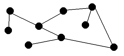
A graph is a data structure which allows us to model
these kinds of relationships. A graph is a collection of vertices (such
as major cities) and edges (roads between those major cities). Any
collection of vertices and edges is a graph. For example, the following
is a graph:

This graph does not demonstrate any noticeable pattern, but from certain
points we can get to other points. Some graphs do have a recognizable
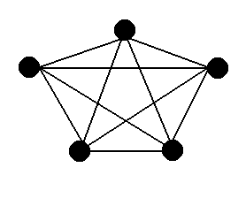
pattern such as:


The first graph is what we call a complete
or fully-connected graph. In a fully-connected graph,
every vertex has an edge to every other vertex.
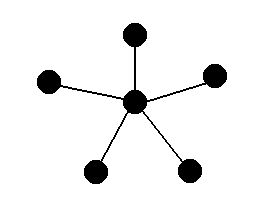
The graph on the right should seem familiar to you. If we bunch up all
of the edges at the bottom so that the center is now on top, this should
look strikingly similar to a generic tree. This is not a coincidence --
trees are graphs. In fact, they are a very specific type of graph: one
without any cycles. A cycle is a sequence of edges that
creates a path back to the vertex it starts at without reusing any of
the edges.
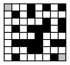
We used cities and roads as an example of what a graph might represent.
Another common use for graphs is to model a maze.

In the case of a maze, the vertices represent each spot which you could
ever be at, and the edges join those spots to all of the spots you could
move to from there. As we will see, how you choose which spot to go to
next could affect what path through the maze you eventually find.
Weighted Graphs
What if we wanted to go from Philadelphia to Charleston? We could go
through Pittsburgh, but what if there is a better way? If we start out
in a more southwestern direction, we might be able to find a faster route
from Philadelphia to Charleston. On the other hand, while there might be
a more direct path, the roads involved might be small slow roads, so the
time that it takes might actually be longer even though the path is shorter.
In a graph, we can factor these details in when we are trying to find the
best way to get from one place to another. Rather than simply indicating
that there is an edge between two vertices, we will also give that edge a
weight. If we are trying to find the fastest path from Philadelphia to
Charleston, then the weight we use might be the expected time it takes on
each part of the trip. If we are trying to find the shortest path, the
weight we use might be the actual length of each part of the trip. We could
also use some combination of these values.
We call this a weighted graph. For convenience, we will say
that the weight will be infinity if there is no edge between two vertices,
and that there will be a weight of 0 for staying at the current node.
Directed Graphs
Again returning to the road analogy, there is the concept of a one-way street.
If you are at the Cathedral Of Learning and need to go to the highway, you
have to use Fifth Ave., but if you are coming from the highway to the
Cathedral Of Learning, you need to use Forbes Ave. instead, because both
streets are one-way.
We might also want to have this type of behavior in our graph. We might
want to be able to go from vertex A to vertex B directly, but not be able
to go from vertex B to vertex A. We call this a directed graph.
In a directed graph we say than an edge goes "from" one vertex "to" another
vertex. If the edge can go both ways then it is an undirected graph. If all
of the edges are undirected then we call it an undirected graph.
A directed graph can also be weighted. It might be really easy to go
directly from vertex A to vertex B, but it might be very difficult (though
possible) to go directly from vertex B to vertex A. In this case, there
would be an edge from A to B and an edge from B to A, but the edge from
B to A would have a much higher weight than the edge from A to B.
How Do We Represent Graphs?
Now that we understand what a graph is, how do we represent them on a
computer. With the Linked List and the Binary Tree it was easy, but graphs
are unstructured. One vertex might be adjecent to every other vertex, but
another vertex might only be adjacent to just that one. (By adjacent, we
mean that there is an edge between them, or that there is an edge from
that one to the other in the case of a directed graph.)
Now when we are doing graphs, sometimes we assume that the vertecies are
connected to themselves. Depending on the problem if they are not automatically
connected to themselves we can draw it in.
There are two common ways of representing graphs. One is called an
adjacency list, the other is called an adjacency matrix.
Adjacency List
An adjacency list representation is essentially an array of linked lists,
one for each vertex, where the linked list contains all of the vertices that
are adjacent to a given vertex, and in the case of a weighted graph, the
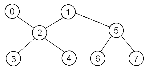
weight between that vertex and each of the others. Suppose we have the
following graph (the naming of the vertices is arbitrary):

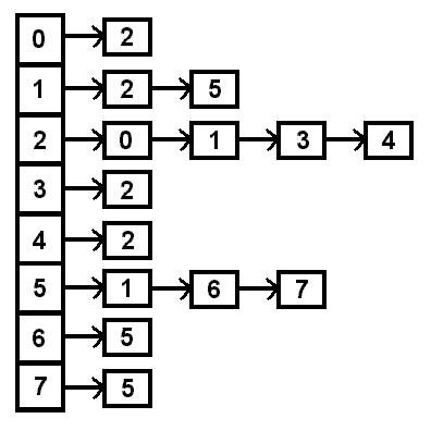
Then our adjacency list would look like:

Why is this? Well, vertex 0 only has an edge with vertex 2, but
vertex 2 has edges with vertex 0, vertex 1, vertex 3, and vertex 4,
so the only item in the list at index 0 is 2, while at index 2 the list
contains 0, 1, 3, and 4. If this were a weighted graph, the nodes of the
list would need to include both the number of the vertex and the cost
to get there. If this were a directed graph, then an edge from 0 to 2 would
not necessarily mean that there would be an edge from 2 to 0.
Adjacency Matrix
Another way we can represent a graph is by using an adjacency
matrix. An adjacency matrix is a table which tells
us if there is an edge between two vertices, and in the case of a
weighted graph, the weight of the edge.
If there are N vertices in the graph, the adjacency matrix will
be an N x N array of integers, where the rows represent the "from"
end of the edge, and the columns represent the "to" end of the edge.
The entry at (i, j) contains the weight of the edge from vertex #i to
vertex #j, or infinity if no such edge exists.
In the case of a bidirectional graph, if there is an edge from vertex #i
to vertex #j there is also an edge from vertex #j to vertex #i, so the
adjacency matrix will be symmetric.
Let's take another look at the graph we used for the adjacency list:

The adjacency matrix for this graph would be:
|
| 0
| 1
| 2
| 3
| 4
| 5
| 6
| 7
|
| 0
| 0
| -
| 0
| -
| -
| -
| -
| -
|
| 1
| -
| 0
| 0
| -
| -
| 0
| -
| -
|
| 2
| 0
| 0
| 0
| 0
| 0
| -
| -
| -
|
| 3
| -
| -
| 0
| 0
| -
| -
| -
| -
|
| 4
| -
| -
| 0
| -
| 0
| -
| -
| -
|
| 5
| -
| 0
| -
| -
| -
| 0
| 0
| 0
|
| 6
| -
| -
| -
| -
| -
| 0
| 0
| -
|
| 7
| -
| -
| -
| -
| -
| 0
| -
| 0
|
Above, "-" means that there is no edge there (the value is infinity).
In this case, the graph was bidirectional, so if you look along the
diagonal, you will see that the matrix is, in fact, symmetric. If this
were a large graph with many vertices, we could save space by only storing
the upper or lower triangle, and use those values as both index (i, j) and
index (j, i).
Also, if you look at this matrix, you will see that we have 0's along the
diagonal, which suggests that vertices are adjacent to themselves. This
is implementation specific -- depending on what you are trying to represent,
you may or may not want to let vertices be adjacent to themselves.
Now, let's take a look at code to implement an adjacency matrix. We will
implement the same methods that the AdjList class has.
Lists Vs. Matrices
We have two ways to represent graphs, so which one should we use?
Well, if the graph is sparse (there aren't many edges), then the matrix
will take up a lot of space indication all of the pairs of vertices which
don't have an edge between them, but the adjacency list does not have that
problem, because it only keeps track of what edges are actually in the
graph. On the other hand, if there are a lot of edges in the graph, or if
it is fully connected, then the list has a lot of overhead because of
all of the references.
If we need to look specifically at a given edge, we can go right to that
spot in the matrix, but in the list we might have to traverse a long linked
list before we hit the end and find out that it is not in the graph.
On the other hand, if we need to look at all of a vertex's neighbors, if you
use a matrix you will have to scan through all of the vertices which aren't
neighbors as well, whereas in the list you can just scan the linked-list of
neighbors.
If, in a directed graph, we ask the question, "Which verticies
have edges leading to vertex X?", the answer is straight-forward
to find in an adjacency matrix -- we just walk down column X and
report all of the edges that are present. But, life isn't so easy
with the adjacency list -- we actually have to perform a brute-force
search.
So which representation you use depends on what you are trying to represent
and what you plan on doing with the graph.
