Return to the Lecture Notes Index
15-111 Lecture 28 (Wednesday, April 4, 2003)
A Quick Review
Okay. Before I dig in to today's topic, "Binary Search Trees (BSTs)", I'd
like to do a quick review of stuff from earlier this semester: searching.
So, if this sounds familiar -- it should be. But, it was o' so long ago.
The "Sequential Search", a.k.a., The "Brute Force Search" and The "Linear Search"
One approach to search for something is just to consider each item, one
at a time, until it is found -- or there are no more items to search.
I remember using this approach quite a bit as a child. I'd open my toy
box and throw each toy out, until I found the one I was looking for.
(Unfortunately, this approach normally resulted in a parental command to
clean my room -- and someitmes quite a fuss).
Imagine that I had a toybox containing 10 items. In the average case,
I'd end up throwing 4 or 5 items on the floor, and my treasured toy
would be the 5th or 6th item -- I'd have to search half of the toy box.
Sometimes, I would find it the first time -- right on top. Sometimes it'd
be the last one -- at the very bottom. And on the balance of occasions --
somewhere in between.
A Quick Look at the Cost of Sequential Searching
So, if, in performing a linear search, we get lucky, we'll find what we
are looking for on the first try -- we'll only have to look at one item.
But, if we get unlucky, it'll be the last item that we consider, and
we'll have had to look at each and every item. In the average case, we'll
look at about half of the items.
Since, the worst case could require looking at each and every item, it
is really easy to see that this seach is O(n). And, the average case
is also linear time -- so, unlike quck sort, this is rough going in most
cases.
The "Binary" Search
But, let's consider a different case for a moment. The case of a sorted,
indexed list. Let's consider, for example, looking for a particular
number in a sorted list of numbers stored within an array or Vector:
| Numbers: |
3 |
7 |
8 |
9 |
11 |
14 |
19 |
25 |
31 |
32 |
| Index: |
0 |
1 |
2 |
3 |
4 |
5 |
6 |
7 |
8 |
9 |
We know that this list is in order. So, we know that there is just as
good a chance that it comes before the "middle" as it does after
the "middle". In other words, whatever number we are looking for
is just as likely to be in the list of numbers with indexes 0-4 as it
is the list with indexes 5-9.
So, we can compare the number with one of the two "middle" numbers,
the number at index 4 or the number at index 5. If it happens to
be the one we're looking for, we got lucky -- and can celebrate.
If not, we'll know better where to look. If it is less than this
"middle" number, it has an index less than the middle number. If
it has an index greater than the middle number, it has an index
greater than the middle number. Either way, we've eliminated half
of the possible places to search. We can search must faster
by considering only those numbers in the right half of the list.
Since this approach decides between searching two sublists, it
is often known as a binary search. Binary means having
two states -- in this case, left and right (a.k.a, less than and greater
than).
To better illustrate this, I'll pseudocode this algorithm recursively,
and then go through it by hand. The recursive algorithm looks like
this:
  public static void searchSortedIntArray (int findMe, int []list, int beginIndex, int endIndex)
  {
    int middleIndex = beginIndex + (endIndex - beginIndex)/2;

    // If the middle point matches, we've won
    if (list[middleIndex] == findMe)
      return true;

    // If it is in the left list, and the left list is non-empty, look there.
    if ( (list[middleIndex] > findMe) && (middleIndex > beginIndex) )
      return searchSortedIntArray (findMe, list, beginIndex, middleIndex-1 );

    // If it is in the right list and the right list is non-empty, look there.
    if ( (list[middleIndex] < findMe) && (middleIndex < endIndex) )
      return searchSortedIntArray (findMe, list, middleIndex+1, endIndex);

    // We're not it and the correct sub-list is empty -- return false
    return false;
  }
Now, to go through it by hand, let's first pick a number in the list:
8. We start out looking at index (9/2)=4, which contains 11. Since 7 is less
than 11, we consider the sublist with indexes 0-3. Since (3/2)=1, we
next consider 7, the valuse at index 1. Since 7 is less than 8, we look
at its right sublist: beginning with index 2 and ending with index 3.
The next "middle" index is 2+(3/2)=3. Index 3 contains 8, so we return
true. As things unwind, that propagates to the top.
Now, let's pick a number that is not in the list: 26. Again, we start
with the vlaue 11 at index 4 -- this time we go next to the right
sublist with indexes 5 through 9. The new pivot point is 7. The
value at this point is 25. Since 26 is greater than 25, we consider
the right sublist with indexes 8 and 9. The new pivot is index 8,
which holds the value 31. Since 26 is less than 31, we want
to look at the left sublist, but we can't, it is empty. Index 26 is
both the middle point, and the left point. So, we return false, and
this is propogated through the unwinding -- 26 is not in the list.
A Careful Look at the Cost of Binary Search
Each time we make a decision, we are able to divide the list in half.
So, we divide the list in half, and half again, and again, until there
is only 1 thing left. Discounting the "off by one" that results from
taking the "pivot" middle value out, we're dividing the list exactly in
half each time and searchong only one half.
As a result, in the worst case, we'll have to search Log2 N
items. Remember 2X = N. So, for a list of
8 items, we'll need to consider approximately 3 of them. Take a look at
the table below, and trace through a list by hand to convince yourself:
| N | Max. Attempts |
|---|
| 1 | 1=(0+1); 20=1 |
| 2 | 2=(1+1); 21=2 |
| 3 | 2=(1+1); 21=2 |
| 4 | 3=(2+1); 22=4 |
| 5 | 3=(2+1); 22=4 |
| 6 | 3=(2+1); 22=4 |
| 7 | 3=(2+1); 22=4 |
| 8 | 3=(2+1); 22=4 |
| 9 | 4=(3+1); 23=8 |
| 9 | 4=(3+1); 23=8 |
| 10 | 4=(3+1); 23=8 |
| 11 | 4=(3+1); 23=8 |
| 12 | 4=(3+1); 23=8 |
| 13 | 4=(3+1); 23=8 |
| 14 | 4=(3+1); 23=8 |
| 15 | 4=(3+1); 23=8 |
| 16 | 5=(4+1); 24=16 |
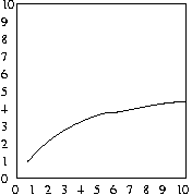
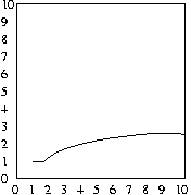
And, as before, the average number of attempts will be half
of the maximum number of attempts, as shown in the plots below:

Worst case of binary search

Average case of binary search
Binary Search: No Silver Bullet
So, instead of searching in O(n) time using a linear search, we can
search in O(log n) time, usng a bianry search -- that's a huge win.
But, there is a big catch -- how do we get the list in sorted order?
We can do this with a quadratic sort, such as Bubble sort,
Selection Sort, or Insertion Sort, in which case
the sort takes O(n2) time. Or, we can use Quick Sort,
in which case, if we are not unlucky, it'll take "n*log n" time. And,
soon, we'll learn about another technique that will let us reliably sort
in O(n*log n) time. But, none of these options are particularly
attractive.
If we are frequently inserting into our list, and have no real reason
to keep it sorted, except to search, our search really degenerates
to O(n*log n) -- becuase we are sorting just to search. And, O(n*log n)
is worse than the O(n) "brute force" search.
Whmmm...there has to be a better way...
Pondering the Big Picture
When we perform a binary search, what we are really doing is creating a
tree of sorts. We'll discuss trees in more detail very soon. So, don't
worry about the details right now. Instead, just think of this tree as
a "decision tree", such as one you might encounter in a business class.
Each time we pick a new number and ask, "Is this it? If not, which
side is it one?" What we are really doing is creating two lists from
the original list, those less than the number and those greater than
the number. Then, we are eliminating at least one of the lists (both
of the lists, if the number happens to be the one we're looking for).
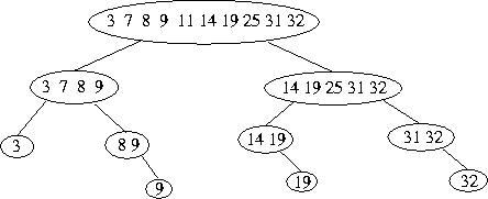
Let's consider our prior example one more time. But, this time, let's
draw out the entire tree, and show the possible sub-lists:

The figure above should highlight the strategy here pretty well:
divided the ordered list into partitions, until we find the right
partition. Each time, we have half as many items to search. Also,
for anyone still haivng difficulty understanding why the search is
O(log n), maybe this helps -- notice the length of the branches with
respect to the number of items in the list. The longest branches
are Log2 n.
Introduction to Binary Search Trees (BSTs)
The next data structure that we'll examine is known as a Binary Search
Tree, most often known simply as a BST. The theory of operation
is going to be basically the same as that of the binary search,
except that it'll be a little more "relaxed".
Instead of building the entire tree in advance, by sorting the list of
numbers using something like quick sort or selection sort, we are going to
build it "as we go along", by inserting the numbers into the tree. This
is very similar to, for example, using insertion sort instead of selection
sort.
But, unlike using insertion sort as the basis for a binary search, we're
going to do something a little faster -- but a little less exact. Let's
take a look:
How Do Binary Search Trees (BSTs) Work?
BSTs are trees. Each node of the tree is much like a node of a
doubly linked list. It contains a value, and references to up
to two other nodes. Each fo these nodes, in turn, contains a value and
a reference to up to two other nodes. We call these other nodes the
left and right children.
The idea is that each node represents some point within a sorted list.
To the left of this point lie values less than it. To the right of this
point lie values greater than it. It is important to realize that
there might be no value in either direction, or the node in that direction
might, itself have children.
But, since this property can be applied recursively, we known that
all of the nodes to the left of a particular node, even if they are
children of (below) another node, are less than the node. The same goes
for all of the nodes to the right.
One way of thinking of this is that each node is the root of
two subtrees: the left subtree and the right subtree. Everything in
the left subtree is less than the root. Everythign in the right subtree
is greater than the root.
The important thing about this arrangement is that we can, as we did
before, work our way form the top (root) of this tree to the bottom,
dividing the list each time, so we can discard all of the possibilities
in one direction or the other.
Constructing a Binary Search Tree
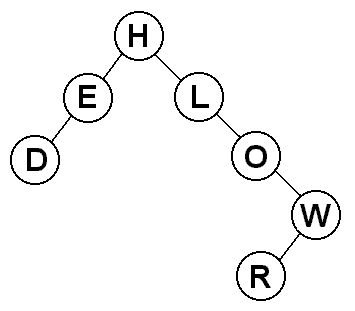
Let's construct a binary search tree using by inserting the letters of
"HELLO WORLD" into the tree one at a time. For convenience, we will ignore
duplicate letters.

How did this work? Let's go through the string one letter at a time.
- "H" - the tree is initially empty, so "H" becomes the root
- "E" - "E" comes before "H", so it goes on the left
- "L" - "L" comes after "H", so it goes on the right
- "L" - "L" is already in the tree, so we ignore it
- "O" - "O" is greater than "H", so it goes to the right of it,
and it is greater than "L", so it goes to the right of that, too
- "W" - "W" is greater than "H", so it goes to the right of it,
it is greater than "L", so it goes to the right of that, and it
is greater than "O", so it goes to the right once again
- "O" - "O" is already in the tree, so we ignore it
- "R" - "R" comes after "H", "L", and "O", so it goes to the right
of all of them, and then it comes before "W" so it goes to the
left of it.
- "L" - "L" is already in the tree, so we ignore it
- "D" - "D" comes before "H", so it goes to the left of it, and it
also comes before "E", so it goes to the left of that, too.
The result is the tree you see. If you look at any node in the tree, you
will see that the binary search tree ordering property holds.
An Example of Using A Binary Search Tree?
Suppose we're looking for the letter F in the "HELLO WORLD" tree.
We can immediately eliminate everything to the right of the H, because we
know that F can't be there because F comes before H. We move on to E,
and we can eliminate everything on its left, because we know that it can't be
there because it comes after E. E's right child is null, so we have
determined that F is not in the tree by only looking at 2 of the 7 nodes.
How Much Does It Cost?
How many nodes do we have to look at in a tree before we know that an item
is not in the tree? To simplify this, we will only look at the best
possible trees of a given size. These best trees are complete and balanced,
meaning that the path from the root to the farthest leaf is at most one
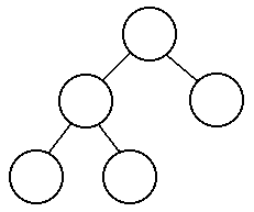
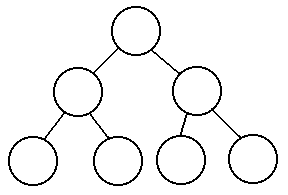
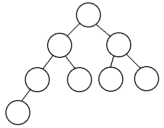
step longer than the path from the root to the closest leaf. The following
are examples of balanced trees:


So how many nodes do we have to look at in the worst case? If there are
N nodes in the tree:
| N nodes
| # looked at
|
| 1
| 1
|
| 2
| 2
|
| 3
| 2
|
| 4
| 3
|
| 5
| 3
|
| 6
| 3
|
| 7
| 3
|
| 8
| 4
|
You can probably see a pattern here. The number of items
you need to look at grows every time we reach a power of 2. We
would only need to look at 4 items for trees with between 8 and 15 nodes
and then we would have to look at 5 items in a tree with 16 nodes. This
is known as logarithmic growth, and we can create a formula for the
number of items we need to look at in a tree with N nodes.
# items = (log2 N) + 1
The Costs of a BST
In a tree with 1,000,000 nodes, we would only need to look at 20 nodes
to insert or find a node. This is a significant improvement over a linear
search and comparable to sorting a list and performing a binary search.
But, in practice, it is much cheaper than sorting a vector, for example
using a insertion sort. This is because, if we can accurately capture the
tree representation with a data structure, we don't need to "push back"
every other node for an insert.
The flip side is that the worst case is bad -- it could degenerate to
a linear search of a linked list. Much like a quick sort, this technique
is not stable -- but, given typical data performs comparably with the
best case.
Now, let's take a look at building a BST class.
The Comparable Interface
As we start developing code to implement Binary Search Trees, we're going
to need a way of comparing different Objects. The Java Comparable
interface provides this functionality in the form of the compareTo()
method. So, instead of dealing with Objects, our trees will store
Comparable Objects -- only those Objects that implement the Comparable
interface. Although you have used the compareTo() method in lab, we
never did formally introduce it in lecture -- so we'll do that now.
The Comparable Interface defines only one method:
int compareTo(Object o).
Let's consider a.compareTo(b). In this case, compareTo() will
return 1 if a is greater than b, 0 if the two are equal,
or -1 if a is less than b.
Remember, the compareTo() method must be defined in each Object that
implements the Comparable interface. It is in this definition where
the implementor of how the particular type of Object is compared.
The Big Picture
Much like our LinkedList and DoublyLinkedList classes,
our BST will require two related classes: a BSTNode to represent the
data and the left and right subtrees, and the BST, itself,
which will contain the root of the tree and all of the methods,
such as insert() and find(), that manipulate it. c
The root of the BST class serves a very similar purpose to the
head of the LinkedList -- it gives us a place to start. And
the left and right references within the BSTNode
are analagous to the prev and next references within a
doubly linked list node. They name other, related, nodes that are part of
the tree structure. And, as before, the data member will be accessible, but
immutable. The other references within the BSTNode will be mutable.
Inserting Into A Binary Search Tree
We already went through the process of building a tree when we created
the "HELLO WORLD" tree, so now let's take a look at some code to perform the
insertion. Since trees are naturally recursive, we will use recursion.
The root parameter in this code is the current subtree, not
necessarily the root of the original tree. We search for the position to
insert the new node, by cutting the original tree in half with each
examination, and determining which half to search. We then call the
insert method recursively on the correct half of the tree, by passing it
either the left child or the right child of the root from the previous
recursive activation.
// "root" here is the root of the current subtree
void BSTinsert(BinaryTreeNode root, Comparable data)
{
   // if the tree is initially empty, the data we
   // add becomes the root of the tree
   if (null == this.root)
   {
      this.root = new BinaryTreeNode(data);
      return;
   }

   // if the current data matches the data we want to
   // insert, it is already in the tree so we ignore it
   if (root.data().compareTo(data) == 0)
   {
      return;
   }

   // if the current data is greater than the one we
   // want to add, we need to go to the left
   if (root.data().compareTo(data) > 0)
   {
      // if the left is null, we can add data there
      if (root.left() == null)
      {
         root.setLeft(new BinaryTreeNode(data));
         return;
      }
      // if not, we need to recursively insert into the
      // subtree on the left
      else
      {
         BSTinsert(root.left(), data);
         return;
      }
   }
   // if the current data is less than the one we want
   // to add, we need to go to the right
   else
   {
      // if the right is null, we can add data there
      if (root.right() == null)
      {
         root.setRight(new BinaryTreeNode(data));
         return;
      }
      // if not, we need to recursively insert into the
      // subtree on the right
      else
      {
         BSTinsert(root.right(), data);
         return;
      }
   }
}
Searching in a Binary Search Tree
As with insert(), this is implemented recursively. It returns
the data, if found, or throws an exception, otherwise.
Comparable BSTfind(Node root, Comparable findMe) throws NotFoundException
{
   // if the current subtree is null, the findMe
   // can't possible be in it
   if (null == root)
   {
      thrown new NotFoundException("Item not found in BST.")
   }

   // if the current data matches findMe, we have
   // found it so we can return it
   if (root.data().compareTo(findMe) == 0)
   {
     return root.data();
   }

   // if the current data is greater than findMe, then
   // if findMe is in the tree it must be to the left,
   // so we will recursively search the left subtree
   if (root.data().compareTo(findMe) > 0)
   {
      return BSTfind(root.left());
   }
   // if the current data is less than findMe, then
   // if findMe is in the tree it must be to the right,
   // so we will recursively search the right subtree
   else
   {
      return BSTfind(root.right());
   }
}
