Heather L. Jones
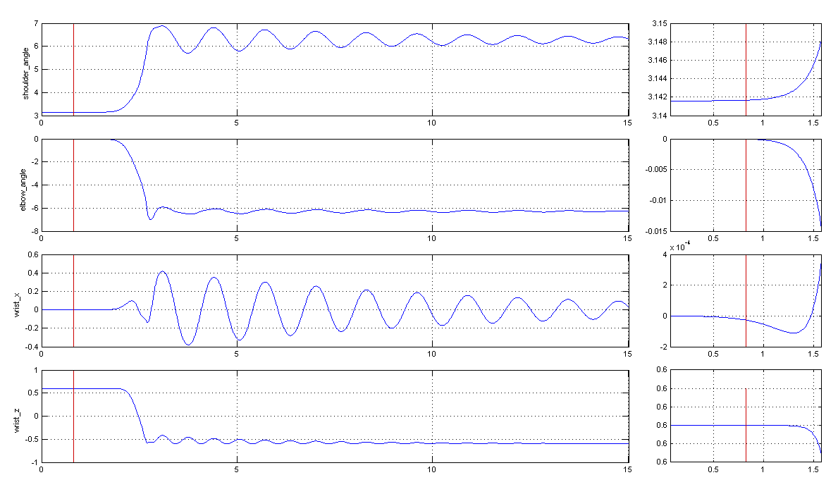
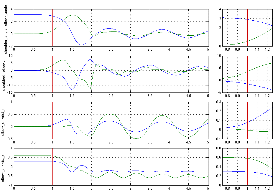
The plots and video below illustrate that I have gotten the simulate, mrdplot and animate code working on my machine. The simulation starts with the arm state [3.14, 0.0, 0.0, 0.0]. No torque is applied to either joint. The plots show shoulder and elbow joing angles, shoulder and elbow joint velocities, elbow and wrist x positions, and elbow and wrist z positions.
If you have trouble seeing the video above, you can also find it here: http://www.youtube.com/watch?v=YhMXYpbh_28
a. To bring the arm to target joint angles of [1.0, 1.0] within ~1 second using a PID controller, the following gains work reasonably well with little overshoot:
| Joint | Shoulder | Elbow | |
| Kp | 1.6 | 9.4 | |
| Ki | 0.18 | 0.06 | |
| Kd | 2.52 | 1.2 |
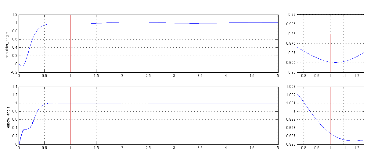
These gains were tuned by hand. There is a slight overshoot in this case, and some oscillation. Increasing the Kd gain would tend to decrease the oscillation, and the Kp gain could be decreased such that the angle levels off closer to the 1 second target. With the time-step used in this case (0.01 seconds), however, small changes tended to cause the system to become unstable, sometimes in unpredictable ways.
To bring the arm to target joint angles of [1.0, 1.0] within ~0.1 second, the following gains were used:
| Joint | Shoulder | Elbow | |
| Kp | 400 | 130 | |
| Ki | 0.08 | 0.02 | |
| Kd | 19 | 6 |
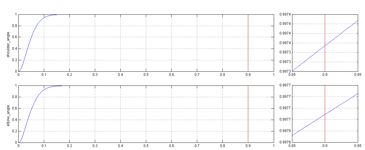
The time-step was changed to 0.01 seconds for this case.
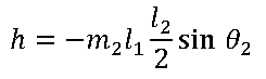
b. The Ki gains can be used to correct steady state error, but they would need to be tuned differently depending on the target configuration. The exact target joint angles can easily be achieved for any target when gravity compensation is added. Because the mass and length of each arm link are known, the torque due to gravity can be calculated for any joint angles. The opposite torques can then be input at the joints. The gravity compensation torques needed are:
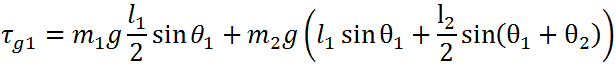
With gravity compensation active, the following gains work well. Note that in this case there are no integral gains.
| Joint | Shoulder | Elbow | |
| Kp | 3.5 | 4.7 | |
| Ki | 0.0 | 0.0 | |
| Kd | 1.81 | 1.2 |
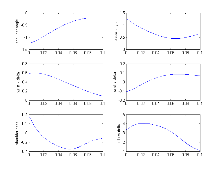
a. The end effector can be moved to an (x,z) target by converting the delta x and delta z between the position at the current time-step and the target into deltas in joint angle space. Torques proportional to these joint angle deltas will drive the end effector toward the target (though not necessarily in a straight line). Torques equal to the joint velocities times a damping factor can reduce or eliminate oscillation around the target. The following plot shows the arm moving to a target at (0.2, -0.5). The Kp gains in this case are both 2, and the Kd gains are both 1.
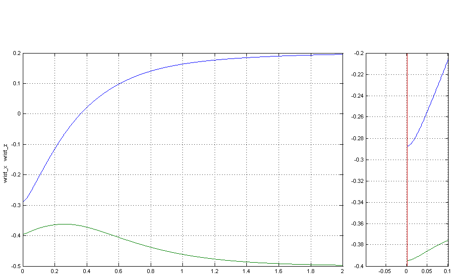
b. A small difference in end effector position in task coordinates (delta x, delta z) can be mapped to a small difference in joint coordinates (delta theta1, delta theta2) using the inverse of the Jacobian. For this problem, the Jacobian is:
where l1 and l2 are the link lengths and each link center of mass is located halfway along the link. This approach fails when the Jacobian becomes singular and cannot be inverted. The plot below shows the delta theta values calculated as the delta x and delta z values and the joint angles change.
c. Given a desired velocity direction in joint space obtained by applying the inverse Jacobian to a position error in task space, the applied torque should move accelerate the joints toward the desired joint velocities. Reasonable performance can be achieved by placing gains on the joint position and joint velocity, though this is purely reactive (except, perhaps for the gravity compensation torque). A feed-forward torque can also be calculated using inverse dynamics. The dynamics of the system can be described as:
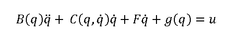
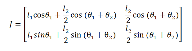
Where u is the control input, q is the joint-space coordinates (theta1 and theta2), g is the gravity compensation torque and F is the coefficient of viscous friction (0.1 for both joints on this robot). The B matrix can be expressed as:
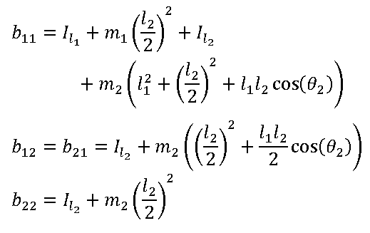 ,
,
The C matrix is:
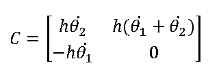
and
As in part (b), a singular Jacobian matrix causes problems for this method, since the joint angle deltas are still calculated using the inverse Jacobian.
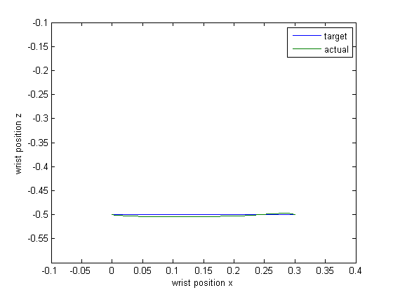
a. To implement trajectory control, the controller function was modified to take the desired wrist accelerations as an argument (the desired wrist position and velocity were already included in the SIM object used by the simulation). The simulate function was also modified to read in a trajectory from a file and pass the appropriate values to the controller. Given the desired positions, velocities and accelerations of the wrist, the desired angles, velocities and accelerations in joint space are calculated. Using the desired joint accelerations and the current joint positions and velocities, a feed-forward torque is calculated using the method described in part 2. Gains on the joint position and velocity error are then used to keep the robot on the trajectory.
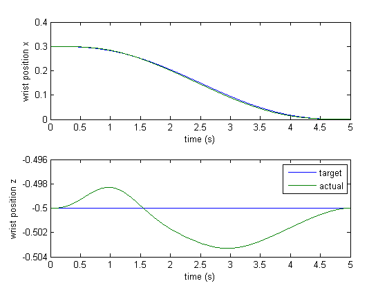
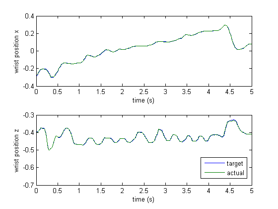
A MATLAB script was used to generate straight-line trajectories in task space. The z components of the wrist position, velocity and acceleration were held at zero. The x component of the wrist position was described by a quintic polynomial, the velocity by a quartic polynomial, and the acceleration by a cubic polynomial (as discussed in class). This ensured that the velocity would be smooth, and the velocity and acceleration would be zero at the start and end of the trajectory. The target start and end positions were set to (-0.3,-0.5) and (0, -0.5), respectively. The trajectory duration was set to 5 seconds.
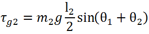
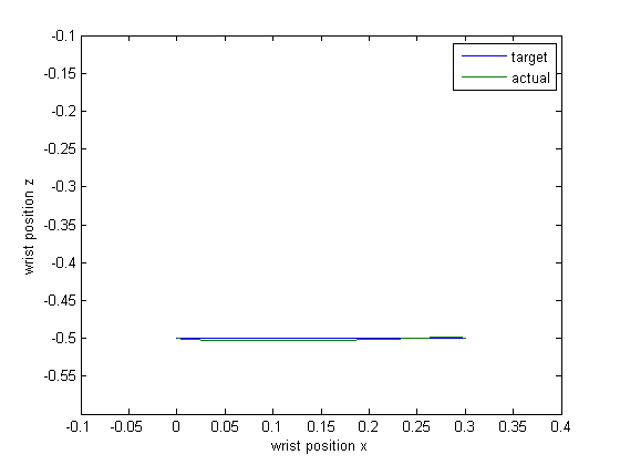
The plots below show the wrist position (x and z) vs. time for the target trajectory and the simulation results. A plot of x vs. z position in task space is also shown.
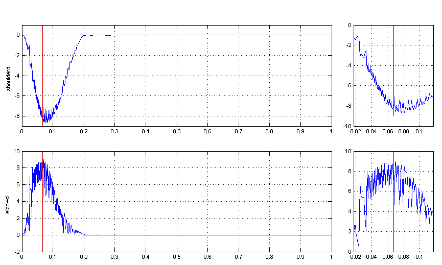
b. The duration of the trajectory from part (a) was decreased from 5 seconds to 0.2 seconds. Initially, the robot was unable to follow the trajectory. When the proportional and derivative gains were appropriately tuned, it had more success. The results shown below are for the following gains:
| Joint | Shoulder | Elbow | |
| Kp | 2000 | 2000 | |
| Kd | 10 | 10 |
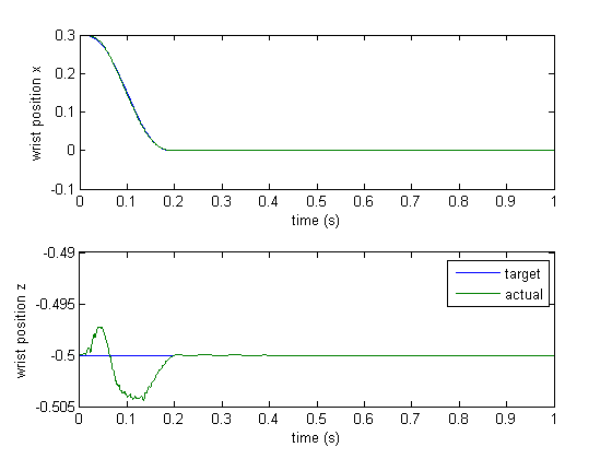
As can be seen in the plots below showing the shoulder (top) and elbow (bottom) joint velocities, the joints reached speeds well above 6 radians/second along this trajectory.
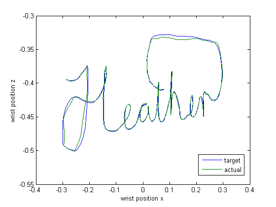
c. A signature (modified so it could be accomplished without lifting the pen) was captured using the mouse.exe program provided with this assignment. The data was loaded into MATLAB, and the trajectory was scaled to fit within the robot's task space (and within a reasonable time). The position data was also smoothed before numerical differentiation was performed to obtain velocities and accelerations. The robot arm was positioned at the start of the trajectory, and it performed well using the gains from part (b). Plots of the target trajectory and simulated results are shown below, along with a video of the robot following the trajectory. Note that the video is slower than real-time.
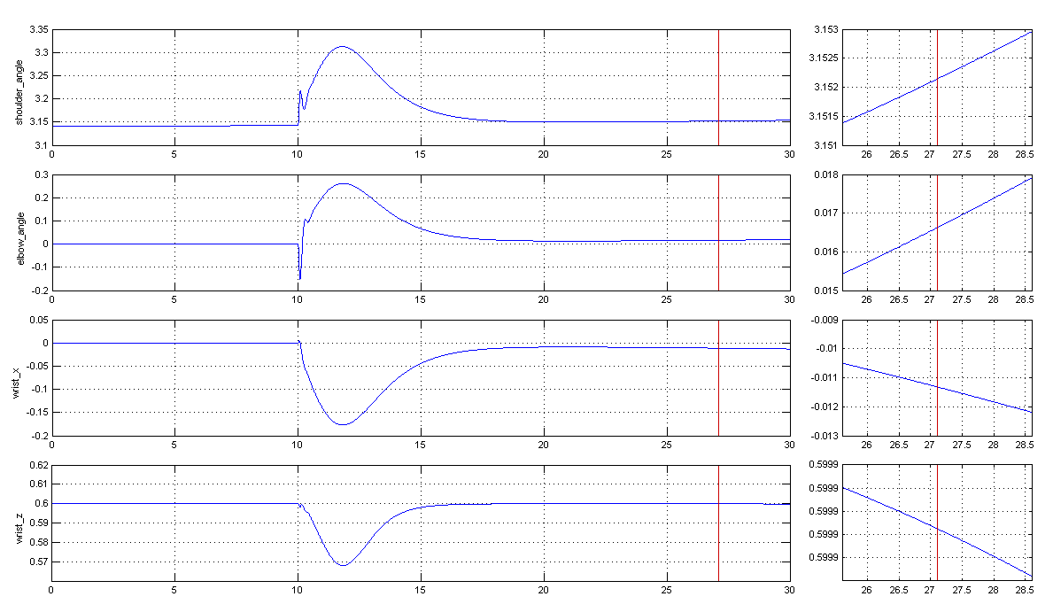
In the following videos and plots, the robot is started with zero velocity in the target position. A disturbance torque is applied to kick the robot out of equilibrium, and the minimum gains needed to return to the target position are found.
With proportional gains of 8.2 on the ankle and 2.4 on the knee joint, the gains are not quite enough to bring the robot fully vertical again before it starts moving away from the target position.
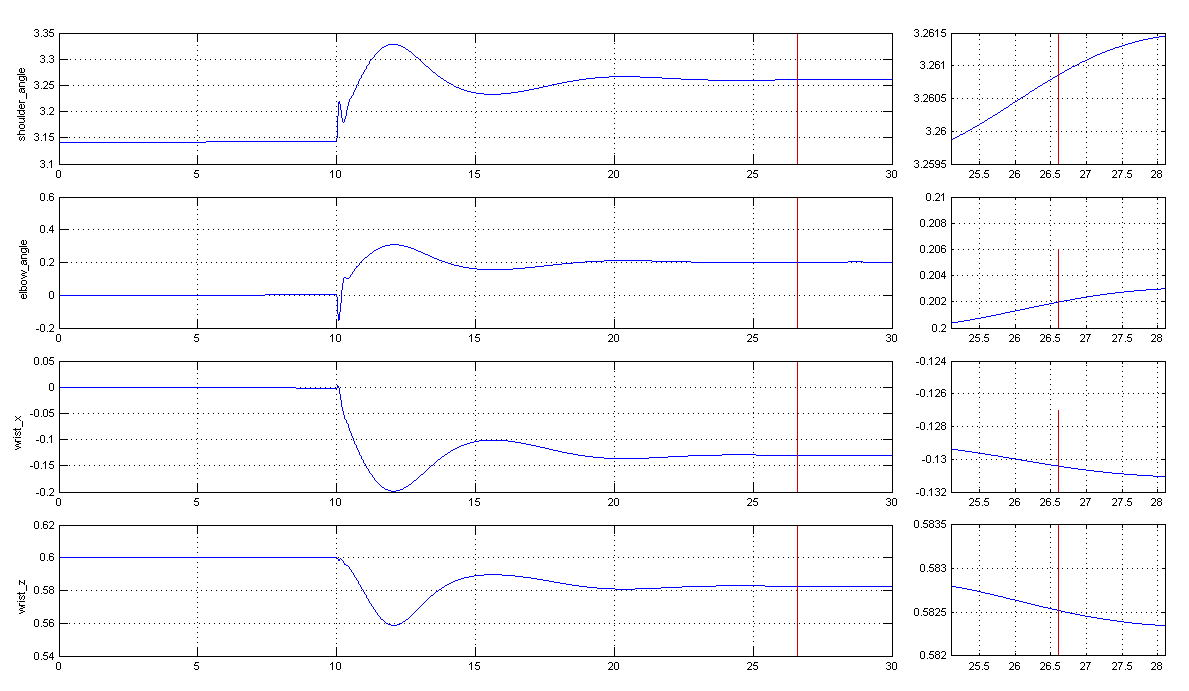
With proportional gains of 8.3 on the ankle and 2.3 on the knee joint, the gains are not enough to bring the robot fully vertical again. It comes to equilibrium away from the target, as can be seen in the plot and video below.
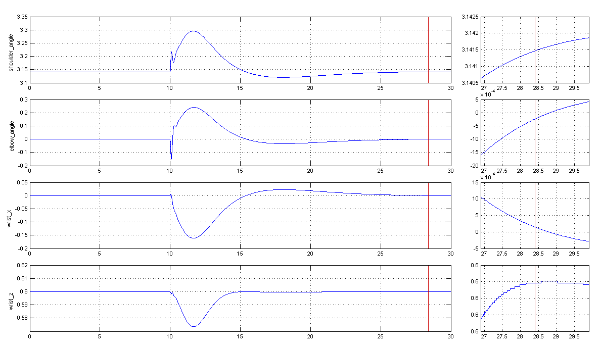
With proportional gains of 8.3 on the ankle and 2.4 on the knee joint, the robot successfully recovers from the disturbance.
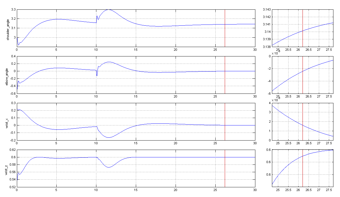
With these gains, the robot can also reach the target position, even if it starts off (in this case at joint angles of 3.0 and -0.5), and it can still recover from the disturbance, as seen in the following plot.
b. When a delay of 0.1 seconds is added to the feedback for the balancing robot, the gains used in part (a) no longer work, and the robot falls down. The plot below shows the joint angles and wrist positions.