Within SEMITIP, surface states are treated as being completely localized at the surface. They influence the band bending through the charge that they carry, which depends on the position of the Fermi-level. Equilibrium (i.e. same Fermi-level) is assumed between surface and bulk states, and the amount of surface charge varies as a function of the radial coordinate in accordance with the radial dependence of the potential. The SEMITIP program solves for the appropriate electrostatic solution such that the final potential profile together with the resulting surface charge all satisfies Poisson's equation.
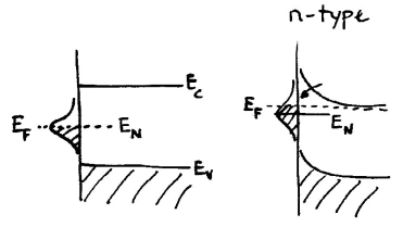
In some early treatments of surface charges a single Gaussian band of states was often assumed, as shown below. In the diagram to the left no semiconductor doping occurs; the surface band is filled with electrons up to some energy known as the "charge neutrality level". This is the energy below which states are neutral when filled and positively charged when empty, and above which they are negatively charged when filled and neutral when empty. The former types of states are known, by definition, as donor-like and the latter as acceptor-like. Now, considering n-type doping as shown in the diagram to the right, some electrons from the conduction band are transferred to the surface band (i.e. since it is lower in energy) as depicted by the arrow. The surface band then acquires negative charge, and in the semiconductor there is positive charge (space charge) left behind from the dopant cores where the electrons have left. The resulting potential profile is as shown in the diagram. Similarly on p-type material downwards band bending results, with the Fermi-level ending up slightly below the charge-neutrality level.
Within the SEMITIP program, the surface charge at each value of the radial coordinate is composed of an integral of the states between the charge-neutrality level and the Fermi-level. (NOTE: This formulation of the integral is actually an approximation, applicable to to zero temperature. VERSION 4 and higher of the program provides the possibility of removing this approximation and including an appropriate Fermi occupation factor in the integral, although for most problems the difference is probably not relevant). One other point to note is the possible extension of the surface states up to energies outside the band gap (i.e. resonant with the bulk bands). Whether or not this phycially occurs depends on the surface under study, i.e. depending on the degree of localization of such resonant states near the surface. The surface states are specified in the function SIG at the bottom of the SEMITIP_Vx.F program. For versions V2 and V3, as written, the surface states do extend outside the bandgap. For versions V4 and V5, as written, the surface states also do extend outside the bandgap, although removing the comment indicators from the first few lines in the SIG routines in these versions will restrict the states to exist only within the bandgap.
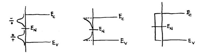
Within the SIG function, the default option is for two possible types of surface bands: separate Gaussian bands of donors and acceptors, or a uniform density of states. These two types appear within SIG as:
      width=fwhm(ID)/(2.*sqrt(2.*alog(2.)))
      sig=-dexp(-1.d0*(ENER-(EN(ID)+ecent(ID)))**2/(2.*width**2))+
     &     dexp(-1.d0*(ENER-(EN(ID)-ecent(ID)))**2/(2.*width**2))
      sig=sig*dens(ID)/(SQRT(2.*pi)*width)
for the two Gaussian bands, or
      sig=dens(ID)
      if (ENER.gt.en(ID)) sig=-sig
for the uniform density. User-specified parameters here are EN (the charge neutrality level, in eV) DENS (the density, in cm-2eV-1 for the Gaussian case or just cm-2 for the uniform density), FWHM (in eV), and ECENT (in eV), with separate values of the parameters for each of the two possible sets of surface state densities that can be input (by default) to the program. If the value of FWHM is zero then the uniform density is employed, otherwise the Gaussian form is employed.
Note that in these code examples, the density of states is negative for energies above the charge neutrality level, and positive below it. These sign specifications determine the character of the surface states: negative for acceptors, and positive for donors. As discussed above, at zero temperature, the total charge density if formed in the program by integrating from the charge neutrality level to the Fermi level to form the negative charge density (arising from acceptor states), or by integrating from the Fermi level up to the charge neutrality level to form the positive charge density (arising from donor states). At nonzero temperature, appropriate Fermi occupation factors are included in the integrals.
Other possibilities for surface states can be formed simply by modifying the SIG routine. For example, to form only a band of donor states (without any acceptors) centered at an energy ECENT below EN, the following code could be used:
      if (ener.lt.en(ID)) then
         width=fwhm(ID)/(2.*sqrt(2.*alog(2.)))
         sig=dexp(-1.d0*(ENER-(EN(ID)-ecent(ID)))**2/(2.*width**2))
         sig=sig*dens(ID)/(SQRT(2.*pi)*width)
      else
         sig=0.
      end if
Here, the density of states is set to identically zero above the charge neutrality level, and it has a Gaussian form below the charge neutrality level. (Note that the normalization of this distribution, integrated over all energies, does not give exactly the value of DENS, due to the truncation of the density at the charge neutrality level. This would only be an issue if the value of FWHM is comparable to or greater than ECENT; in that case, a slightly more complex normalization of the SIG value, i.e. employing an error function, would be needed). As another example, to form two bands of donor states, one centered at ECENT below EN and the other at 2*ECENT below EN, then the following code could be used:
      if (ener.lt.en(ID)) then
         width=fwhm(ID)/(2.*sqrt(2.*alog(2.)))
         sig=dexp(-1.d0*(ENER-(EN(ID)-2.*ecent(ID)))**2/(2.*width**2))+
     &       dexp(-1.d0*(ENER-(EN(ID)-ecent(ID)))**2/(2.*width**2))
         sig=sig*dens(ID)/(SQRT(2.*pi)*width)
      else
         sig=0.
      end if
Similarly, other distributions of surface states can be modeled, simply by modifying the SIG function.
Within the default configuration of the SIG routine and the main calling programs, the user can input parameters for two different sets of surface states. Each set will have its own values of the EN, DENS, FWHM, and ECENT parameters. If nonzero values of DENS are input for both sets of surface states, then the program will combine these two sets in order to form a resultant, combined distribution of surface states. The integrated charge density for each distribution is formed, an overall charge neutrality level for the combined distribution is located, and then the integrated charge density for the combined distribution is obtained. (This procedure for properly combining the two sets of surface states was actually not performed correctly in versions 6.0 and 6.1 of the surfrho.f and surfrhomult.f routines, but it was corrected in version 6.2 and later of these routines).