Computation of Tunnel Current

The computation of tunnel current in the SEMITIP program follows the method described in Refs. 1 and 2. In Ref. 2, the Tersoff and Hamann approximation (Ref. 3) is employed in order to obtain the tunnel current from a specific region of the sample surface, i.e. as appropriate for a sharp probe tip. However, the manner in which this approximation was implemented in the theory (i.e. Eq. (A8) of Ref. 2) was a bit ad hoc. Thus, a more rigorous derivation was developed in Ref. 4, as described below. The resulting formula for the tunnel current differs slightly from that given by the combination of Eqs. (A5), (A6) and (A8) in Ref. 2.

We start with Eq. (5) of Ref. 1 for the probability of tunneling (which is based on earlier work of Duke and of Bardeen), but not assuming that the quantum numbers necessarily involve parallel wavevector,

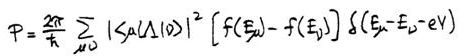where μ labels states of the sample and ν labels states of the tip. The quantity immediately to the right of the summation sign is the matrix element (squared) for the process. Following Tersoff and Hamann, we take for the states of the tip

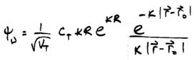and for the sample

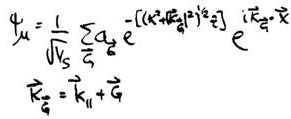where V_S and V_T are normalization volumes for the sample and tip, respectively. Further following Tersoff and Hamann, the matrix element is then found to be

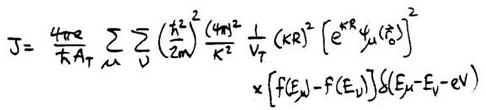
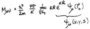where we define here the sample wavefunction at the location of the tip apex, ψ_μ(x,y,s) for tip-sample separation s. We use this quantity, rather than the wavefunction evaluated at the tip center, to compare with experiment since it is the most physically meaningful in terms of its magnitude. Substituting into the equation for the tunneling probability, and taking the current density to be 2eP/A_T where the factor of 2 is for spin and A_T is an effective tip area, the current density is found to be

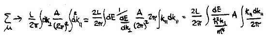
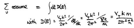
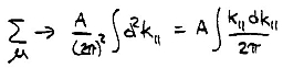
The summation over sample states μ is evaluated as

where L and A are a normalization length and area, respectively. For the summation of tip states we consider states in a the 3D tip volume,

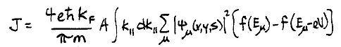
Substituting into the expression for current density, taking A_T=πR², and setting the wavevector in the tip to be k_F, the Fermi wavevector, we find finally

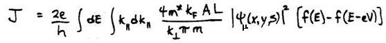It is this expression for the current that is evaluated in the SEMITIP program. This result differs by a factor of (k_F/κ)² compared to that in Ref. 2, but the magnitude of this factor is of order unity in any case. In the above expression the subscript μ on the wavefunction refers to the parallel and perpendicular wavevector values for each state. The parallel part of the wavefunction, when squared, just yields a factor of 1/A which cancels the factor of A in the expression, and similarly the factor of L is cancelled by the normalization of the perpendicular part of the wavefunction. The above expression is applicable for the case of sample states that are extended in the z-direction (i.e. perpendicular to the surface). For states that are localized in the z-direction, we have for the summation over sample states

As above, we substitute into the expression for current density, take A_T=πR², and set the wavevector in the tip to be k_F. Also, we sum over all localized states for a given value of the parallel wavevector. We thus find

As for the extended state case, the parallel part of the wavefunction yields a factor of 1/A which cancels the factor of A in the expression. And again, this expression for J differs from the one in Ref. 2 by a factor of (k_F/κ)².

As just described, the current through localized states refers to localized states that are obtained by solving Schrödinger's equation in the effective-mass (envelope function) approximation, i.e. states that result from band bending in the semiconductor. However, for true surface states the same formula can be used. In that case one does not know the value of the wavefunction squared from an effective-mass treatment, but this value can be estimated as being roughly the inverse of a length over which the wavefunction is localized (e.g. approximately a unit cell length, for highly localized surface states).

One issue to bear in mind when considering the magnitude of the computed tunnel current compared to experiment is the neglect of the image potential in the computation, as discussed in Ref. 1. To account for the image potential, to lowest order, the computed currents should be multiplied by a factor of about 1000.

References:
1. R. M. Feenstra, Y. Dong, M. P. Semtsiv, and W. T. Masselink, Influence of Tip-induced Band Bending on Tunneling Spectra of Semiconductor Surfaces, Nanotechnology 18, 044015 (2007). For preprint, see http://www.cmu.edu/physics/stm/publ/74/.
2. Y. Dong, R. M. Feenstra, M. P. Semtsiv and W. T. Masselink, Band Offsets of InGaP/GaAs Heterojunctions by Scanning Tunneling Spectroscopy, J. Appl. Phys. 103, 073704 (2008). For preprint, see http://www.cmu.edu/physics/stm/publ/79/.
3. J. Tersoff and D. R. Hamann, Phys. Rev. B 31, 805 (1985).
4. S. Gaan, G. He, R. M. Feenstra, J. Walker, and E. Towe, Size, shape, composition, and electronic properties of InAs/GaAs quantum dots by scanning tunneling microscopy and spectroscopy, J. Appl. Phys. 108, 114315 (2010). For preprint, see http://www.cmu.edu/physics/stm/publ/93/.