Workshop 6 The Central Limit Theorem for Census Data

In this workshop, we will analyze the census data in your casebook (you can find it in your case book floppy or you can directly open it from the R: drive) and explore the real meaning of central limit theorem.

The following part will briefly show you how the distributional shape changes when the sample size changes. The notes show you the basic operations in Mintab, which are useful for solving the questions. You need to do more in getting simulation results and write in details your findings when you work on your homework.

STEP 1: Open the data set.

Note: you can open your data set either from your floppy or r:\academic\90786\chatterjee et all\census1.dat). I have ever shown you how to open a text data file in excel, how to partition the plain text file into columns, and how to read the columns in Excel program. This time we will use Minitab to complete the similar task.

From Minitab File Menu, Click File>Other Files > Import Special Text

You will see such a pop-up dialog

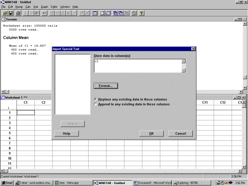
Note that there is only one column data in the plain text file (you can open any plain text in your Wordpad or any other word processor. In this data set you will see only one column.) So you input C1 as the column name in your Minitab worksheet to store the data.

( If you want to use the Minitab program to read in data from a multi-column plain text file, just simply select multiple columns in the pop-up dialog to store every column in the worksheet. Remember, if you only select one column, the program will read the first element of every row in the plain text file and put it in the selected column.)

Click OK
Tell the program where is your input plain text file. In this case, it is or r:\academic\90786\chatterjee et all\census1.dat
You will see the data read in column 1.

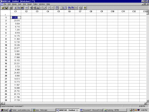
Step 2: Let us have a look at the descriptive statistics and histogram of the data set

· In Minitab, from Stat>Basic Statistics>Descriptive Statistics]

· Select Column, for which you want to compute descriptive statistics

OUTPUT: Mean of C1 = 19.897

400 rows read.

5000 rows read.

Descriptive Statistics

Variable N Mean Median TrMean StDev SE Mean

C1 5000 19.897 16.990 18.709 12.573 0.178

Variable Minimum Maximum Q1 Q3

C1 0.292 220.835 12.123 24.418

· In Minitab, select Graph>Histogram Click ok

· Choose column 1

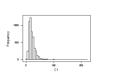
Obviously, the original data set is highly skewed.

Step 3: Understand the real meaning of Central Limit Theorem

The skewness of the original dataset is quire apparent. According to Central Limit Theorem, the probability distribution of will appear to be more and more normal in shape as the sample size increases.

So let us have a look if the shape skewness improves when the sample size increases from 1 to 3.

· Sample 200 observations from the original dataset.

In Minitab, select Calc>Random Data>Sample from Column, then choose Column 1

As the sampling source and Column 2 to store the output.

Click Ok. You will see 200 sampled observations show up in column 2.

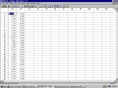
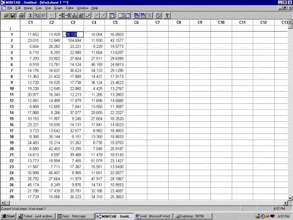
· Continue to sample 200 observations in C3, C4, so we have 600 sampled observations. Each row of C2, C3 and C4 is a sample with sample size 3.

· For each row, compute :

In Minitab, select Stat>Row Statistics

Select ‘Mean’ from statistic, select c2, c3, c4 as input variables, tell the program that you want it to store the mean of every row in c5

Click ok.

· Descriptive statistics

Descriptive Statistics

Variable N Mean Median TrMean StDev SE Mean

C5 200 19.589 18.234 19.023 6.848 0.484

Variable Minimum Maximum Q1 Q3

C5 8.165 46.970 15.005 22.589

Note: The difference between Mean and Median is reduced from 3 to 1.5 when we increase the sample size from 1 to 3. This gives us a sense that the skewness is reduced by increasing the sample size.

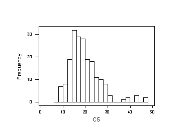
· Histogram

Histogram is always the most often used, direct way to explain the change of distribution shapes.

In this case, when sample size increases to 3, you see the apparent improvement of skewness.