Here is my macro

MBS:

7.97 (25 points)

Sampling error, or “estimation error”, refers to the degree to which a sample statistic differs from the population parameter that the statistic estimates. So, for example, if a poll reports that “61% of the public supports a program of national health insurance”, but in fact the true population parameter (the percentage of the public that supports a program of national health insurance) is 63.42%, the sampling error is +2.42%. Of course, in practice we do not generally know the exact sampling error, since determining it requires knowing the value of the population parameter (and if we knew that, why would be estimating it from a sample, anyway?). Through the use of confidence intervals, however, we can place a bound on the sampling error, thereby giving a fairly reliable range within which the population parameter is expected to fall.

Nonsampling error refers to flaws in the design or implementation of the sampling process, or the interpretation of the results, that could cause unreliability in the conclusions. At least in theory, such error is avoidable with the proper controls and design of an experiment. Sampling error, on the other hand, is unavoidable whenever conclusions are drawn about a population based on characteristics of a sample of that population.

Common types of nonsampling error are discussed in the text on pages 307-308. The quote from Time magazine refers specifically to the following types of nonsampling errors:

· Loaded questions: a question that is worded in such a way as to suggest a particular answer or to influence subjects’ responses would induce bias.

· Interviewer errors: a “sloppily worded question” might be the result of interviewer error.

· Understanding the concepts/Lack of knowledge: when a question evokes complex feelings on the part of the respondent, but permits only a simple answer, the data may be unreliable for the purpose of accurately measuring a subject’s position.

MBS Case 7.3: Sampling Error vs. Nonsampling Error (25 points)

a. Literary Digest Presidential Election poll

Nonsampling error here can be attributed to two main causes: sampling operations and noninterviews.

(1) Sampling Operations: The sampling operations described here would produce biased results. Because republicans and democrats tended to be divided along economic lines, the sampling process would have to produce a sample in which the economic composition was representative of the economic composition of the voting public. That is, a wealthy person would have to be no more likely to be part of the sample than would a poorer individual. However, by obtaining a list of subjects “from sources such as telephone directories, club membership lists, magazine subscriptions, and car registrations,” the sample was almost certain to over-represent wealthy people. This is consistent with the (extremely flawed) result of the poll. Notice that the sources were also likely to produce a predominantly male sample. An alternative sampling method that would reduce the bias would have to address this unbalance in the economic composition of the sample. For example, rather than using telephone directories and the like to obtain the list of subjects, a random sample might be drawn from voter registration data.

(2) Noninterviews: By relying on voluntary response to mail questionnaires, the sampling process suffered from the problem of nonresponse. Although the response rate here was 24%, it may be that those who respond differ from those who do not in ways that may be relevant to the outcome. An alternative sampling method that would reduce the error might be to include a monetary incentive with the questionnaire (see discussion on top of page 307), and/or to follow-up nonresponses to try to obtain responses to the questions.

b. Larry King 900-number

Again, the likely source of nonsampling error is the method of obtaining the sample, or the “sampling operations”. The 900-number method would certainly not produce a random sample; particularly with respect to such a politically and emotionally charged issue. Respondents are actually charged $0.50 here to take part in the survey. Obviously, only people who feel particularly strong about the matter will take the time, effort, and money to respond. Furthermore, there is no way to control “cheating” – that is, particular callers could call in several times in an effort to skew the results. Also, the question was somewhat “loaded” in that viewers were almost certainly influenced by the preceding discussion on the show. Finally, the “population” itself is limited to viewers of the Larry King Live show, which is not necessarily representative of the public at large. Just about any alternative sampling method would be likely to reduce this bias!

Chattergee – Reporting of Sexual Partners (25 points)

Give an example to show that the median number of sex partners of males could be 4 and the median number of sex partners of females could be 1. Note that in your example the mean number of sex partners must be the same for males and females.

Consider the matrix below, where 12 women and 12 men are represented by the numbers 1-12 across the top and left side, respectively. The entries in the matrix indicate whether the particular man and woman have been sexual partners. For example, the “0” in cell (1,5) indicates that Man 1 and Woman 5 have not been sexual partners, while the “1” in cell (8,5) indicates that Man 8 and Woman 5 have been partners. The far right column totals each man’s interactions with the women, while the bottom row totals each woman’s interactions with the men. Notice that the total interactions of men and women obviously must be equal (here, both totals equal 49) since each interaction for a man with a woman is also an interaction for a woman with a man. Since there are 12 men and 12 woman, the mean number of interactions are also equal (here, just over 4 interactions). The median number of interactions for men, however, is 4; while for women it is 1.

Women

Men-Total

Interactions

Men

5

Median - Women

Women

Total Interactions

Median - Men

Prepare and use a Minitab macro to simulate 1000 replications of calculating the maximum of 15 observations from a normal distribution with mean 500 and standard deviation 100. Give descriptive statistics and a histogram fro the 1000 maxima. (25 points)

Here is my macro. Yours may not be exactly the same, but should accomplish the same result.

GMACRO

Normal15

Do k1=1:1000

Random 15 c1;

Normal 500 100.

Let c2(k1)=MAX(C1)

Enddo

ENDMACRO

With each repetition of the DO loop, the constant k1 is incremented by 1. 15 observations from a normal distribution with m = 500 and s = 100 are generated in column 1, and then the maximum of the 15 observations is put into column 2, in the next empty cell. Thus, after the macro is finished running, column 2 contains the 1000 maxima. Now we can run the descriptive statistics on column 2.

Descriptive Statistics

Variable N Mean Median TrMean StDev SE Mean

Maximum 1000 672.72 669.16 671.24 55.77 1.76

Variable Minimum Maximum Q1 Q3

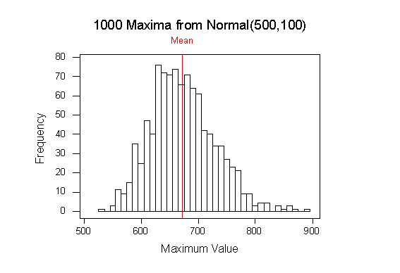
Maximum 527.26 885.86 633.51 707.96