90-786 Homework 1 Answer Key

Problems to be Handed In:

MBS

1.25 (10 points)

a. All major U.S. firms.

b. Job-sharing availability

c. 1,035 firms

d. The agency is interested in making a generalization from the sample of 1,035 firms to the population of all U.S. firms regarding the availability of job-sharing opportunities for workers.

2.25 (15 points)

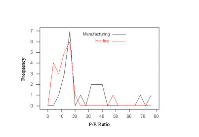
a. Here is one graph that would work:

b. The P/E ratios in manufacturing firms appear to exceed the P/E ratios in holding firms. Notice that you can verify this by looking at the descriptive statistics for each: the mean P/E ratio among manufacturing firms is 26.75, while among holding firms it is 12.70.

2.38 (15 points)

a. The mean number of sites per county is 5.24, the median is 3 and the mode is 2. The mean exceeds the median, indicating that the data is skewed to the right. Thus, the more “extreme” values among the data are large. Half of the counties have three or fewer sites, and more counties have two sites than any other number. TIP: to find the mode, use the cross-tabulation or tally command under the Stat menu, Tables submenu.

b. The largest measurement in the data set is 48. TIP: to make it easy to find a particular point in the data like this, simply use the SORT command under the Manip menu.

c. The descriptive statistics before the deletion (all 75 values) are:

Descriptive Statistics

Variable N Mean Median TrMean StDev SE Mean

C1 75 5.240 3.000 4.149 7.244 0.837

Variable Minimum Maximum Q1 Q3

C1 0.000 48.000 1.000 6.000

After deleting the outlier:

Descriptive Statistics

Variable N Mean Median TrMean StDev SE Mean

C1 74 4.662 3.000 3.955 5.274 0.613

Variable Minimum Maximum Q1 Q3

C1 0.000 25.000 1.000 6.000

The deletion did not change the median or the mode. However, the mean dropped from 5.240 to 4.662.

2.106 (15 points)

a.

Character Stem-and-Leaf Display

Stem-and-leaf of price N = 45

Leaf Unit = 0.10

4 0 3444

(26) 0 55555555566666667777788889

15 1 00011222334

4 1 77

2 2

2 2

2 3

2 3 9

1 4

1 4 7

b. The ADA approved brands’ leaves are underlined.

c. The ADA brands are concentrated among the lower-priced brands.

CHS – Stock Mutual Funds Case (45 points total)

1. Descriptive Statistics

Descriptive Statistics

Variable N Mean Median TrMean StDev SE Mean

FIVEYR 185 14936 14570 14824 2659 196

RETURN92 185 7.351 8.000 7.275 7.845 0.577

Variable Minimum Maximum Q1 Q3

FIVEYR 9426 24161 13410 16410

RETURN92 -14.000 41.000 3.000 12.000

Mean five-year performance is $14,936; mean 1992 return is 7.351%.

2. Comparison to S&P 500: The means for both the five-year performance and the 1992 return fall below that of the S&P 500. This suggests that (overall) the funds studied here perform worse than S&P 500.

3.
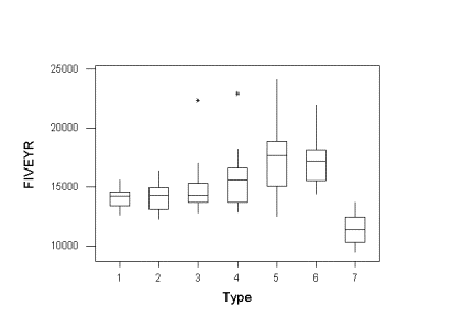
Five-year performance boxplots:

4. Descriptive statistics by type of fund:

Descriptive Statistics

Variable Type N Mean Median TrMean StDev

FIVEYR 1 25 14069 14222 14067 816

2 17 14160 14259 14139 1186

3 32 14642 14301 14413 1711

4 25 15536 15593 15334 2150

5 20 17331 17674 17224 2917

6 37 17220 17182 17117 1974

7 29 11381 11337 11367 1257

RETURN92 1 25 7.440 8.000 7.391 3.675

2 17 9.412 9.000 9.600 3.483

3 32 8.625 7.500 8.571 4.463

4 25 10.52 9.00 10.35 6.31

5 20 8.15 9.50 8.00 8.71

6 37 10.92 12.00 10.42 9.15

7 29 -3.172 -3.000 -3.037 5.029

The mean five year return increases steadily from type 1 (balanced) through type 5 (aggressive-growth), remains approximately the same for type 6 (small-company) funds, and then drops dramatically for type 7 (international and global). With the exception then of type 7 funds, performance on average does better when moving from the less risky to the more risky type of funds.

The standard deviation follows the same pattern as the mean, indicating that those types of funds with the potential for the largest gains also exhibit the potential for the largest losses.

5. Funds of types 3 & 4 both have outlier observations, as indicated by the “*” symbol on the boxplot. These represent extreme values of the measured variable.

The fund types with the more variability in their performance, in general, appear to offer a higher return. This is illustrated by the fact that the boxes with a “wider spread” are also “higher” on the plot.

6.

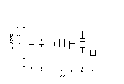
One year performance boxplots:

In general, the variability of the fund types again increases with better performance, although the pattern is not as evident here as in the five year plots. Notice that again there are two categories of funds with outlier observations; however, now it is type 2 and type 6, neither one of which had outliers among the five year observations.

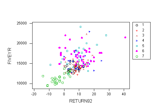
Below is a scatter plot of one year versus five year performance. (It was not necessary to do the plot in color, but may be easier to see the patterns among group types this way.) The points of the scatter plot go vaguely from the lower left to the upper right of the box, suggesting that there is some relationship between short-term and long-term performance. Notice that, as we saw with the boxplots, there is wider variability among the “best” performers (the points are more spread out in the upper right area).

MBS Practice Problems:

2.39 a. The median gives the point in the data that is “in the middle”. Thus, 50% of the observations are below, and 50% above, the median. The median age of 30 in 1980 means that half the population was below 30 and half above, while in 2000 half of the population is expected to be below 36. This suggests that the population of the U.S. is aging.

b. The shift in the median age would mean that a proportionately smaller part of the population is among the industry’s target market. (Notice that this does not necessarily mean that their market is shrinking in absolute terms, as this would also depend on population growth overall.)

2.41 a. Skewed right.

b. Skewed left – more extreme observations to the right of the distribution.

c. Skewed right – more extreme observations to the left of the distribution.

d. Hopefully skewed left! But probably symmetric.

e. Probably symmetric, but you could probably make an argument for any of the three distributions.

f. Skewed left.

2.54 a. range = 3-0=3, s² =1.3, s=1.1402.

b. same as a

c. same as a

d. there is no effect

2.67 a. The empirical rule is not appropriate, since the distribution is not mound-shaped and symmetric.

b. (-1.107, 6.205) Based on Chebyshev’s Rule.

c. 95.9% (47 of the 49 firms).

d. 1.8 months (the mean of the firms that filed a prepackaged plan).

2.68 The mean is 5.24, and the standard deviation is 7.244.

c ± s = (-2.044, 12.484). Seventy of the observations fall in this interval, or 93.3%. This is more than the 68% for the Empirical Rule, and at least 0 for Chebyshev’s Rule.

c ± 2s = (-9.248, 19.728). Seventy-one observations, or 94.7%, are in this interval. This agrees with at least 75% from Chebyshev’s Rule and is very close to the 95% of the Empirical Rule

c ± 3s = (-16.492, 26.972). 98.7% of the observations are in this interval. This is close to “almost all” of the Empirical Rule, and agrees with Chebyshev’s Rule of 89%.

2.72 a. We are given that the distribution is mound-shaped, so the Empirical Rule applies. We know that 1.84% is 2 standard deviations below the mean. The Empirical Rule tells us that approximately 95% of the observations will lie within 2 standard deviations of the mean and, consequently, approximately 5% will lie outside that interval. Since a mound-shaped distribution is symmetric, approximately 2.5% of the day’s production of batches will fall below 1.84%.

b. If the data are actually mound-shaped, it would be extremely unusual (less than 2.5%) to observe a batch with 1.80% zinc phosphide if the true mean is 2.0%. Thus, if we did observe 1.8%, we would conclude that the mean percent of zinc phosphide in today’s production is probably less than 2.0%.