F6 Muffler

Fluid #6: 3D Exhaust Flow Through A Muffler

Introduction: In this example you will model exhaust flow with a given inlet velocity.

Physical Problem: Compute and plot the velocity and pressure distribution over the length of the exhaust.

Problem Description:

	Exhaust at 0.5 m/s flows through the given manifold. Calculate the distribution of the pressure and velocity of the air exiting the manifold.
	You are required to hand in print outs for the above.
	Figure:

Front View:

NOTE: BOTH OF THE IMPEDANCES WITHIN THE MUFFLER ARE 0.01 m THICK. This is because ANSYS does not allow them to be infinitesimally thin.

STARTING ANSYS

	Click on ANSYS in the programs menu.
	Select Interactive.
	The following menu that comes up. Enter the working directory. All your files will be stored in this directory. Also enter 64 for Total Workspace and 32 for Database.
	Click on Run.

MODELING THE STRUCTURE

	Go to the ANSYS Utility Menu
	Click Workplane>WP Settings
	The following window comes up

	Check the Cartesian and Grid Only buttons
	Enter the values shown in the figure above.

In this problem we will model the muffler as a block of air, then model the two volumes defining the impedances within the muffler, then subtract the volume of the impedances from the block of air defining the muffler. At this point we will then apply fluid flow to the inlet of the muffler and see how the flow is impeded due to the muffler’s shape.

	Now, we will create the model.
	Click Preprocessor>-Modeling-> and create a cylinder to define the basic shape of the muffler.
	NOTE: It makes the creation of any 3 dimensional shape easier to go to the ANSYS Main Menu (the top bar) and select PlotCntrls>Pan Zoom Rotate and select the Isometric view (ISO). This simply allows you a better view of the volumes as you form them.
	Now, go to Preprocessor>Modeling>Delete>Volumes Only and click the cylinder just created.
	Click Preprocessor>Modeling>Create>Areas>Rectangle>By 2 Corners and create the area defining the inlet to the muffler. (A circle with radius 0.03 m at the origin)
	Then go to Preprocessor>Modeling>Operate>Boolean>Overlap>Areas and overlap the inlet to the corresponding face of the muffler.
	Now, move the Workplane to the face of the muffler farthest from the origin. Do this by selecting (on the top bar) Workplane>Offset WP by Increments…. At this point, make sure the slider at the top defining the number of snap increments it moves is set to 1 and click the +Z button 3 times. This should positiono the Workplane directly at the end of the muffler. Click OK.
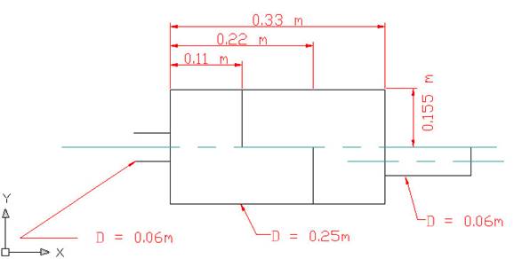
	Now create the area defining the outlet for the muffler. The outlet is a circle of radius 0.03 m offset 0.03 m in the –Y direction. (These dimensions can be extracted from the AutoCAD Drawing in the introduction)
	Again, Overlap the area just created with its corresponding face. (the exit face of the muffler)
	Now create an “arbitrary” volume defined by all areas.
	This new volume is the muffler, complete with inlet and outlet.
	Once the primary muffler volume is finished, move the working plane 0.11 m (the snap increment) along the Z axis such that it’s situated at the base what will be the beginning of the impedance closest to the origin.
	Once the plane is in place, create the volume to be subtracted from the muffler. (Use Preprocessor>Modeling>Create>Volumes>Block>By 2 Corners and Z ) Since only the top half of the muffler needs to be removed in this particular slice set the height to a positive value and the width such that the entire top hemisphere of the volume is included. These dimensions were sufficient for the original model:

Position: (-0.3, 0)
Width = 0.6

Height = 0.3

Depth = 0.01

Now shift the working plane another 0.11 m away from the origin and create the volume to form the other impedance. These dimensions were sufficient for the original model:

Position: (-0.3, 0)
Width = 0.6

Height = -0.3

Depth = 0.01

	Once the impedance volumes have been created, go to Preprocessor>Modeling>Operate>Boolean>Subtract.
	Click the Cylindrical volume, then OK, then select the two impedance volumes and Click OK. This should remove the volumes such that both impedances are subtracted from the larger volume and there is only one volume now.
	The spaces where the impedances would be are now empty volumes. This is because the muffler cylinder is defined as a section of air. This air never penetrates the impedances, so the volume of air is represented as a large cylinder with the impedance sections removed.
	At this point, the finished model should look like this: (If you plot lines, not volumes)

The modeling of the problem is done.

ELEMENT PROPERTIES

SELECTING ELEMENT TYPE:

· Click Preprocessor>Element Type>Add/Edit/Delete... In the 'Element Types' window that opens click on Add... The following window opens:

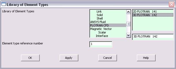
· Type 1 in the Element type reference number.

· Click on Flotran CFD and select 3D Flotran 142. Click OK. Close the 'Element types' window.

· So now we have selected Element type 1 to be a Flotran element. The component will now be modeled using the principles of fluid dynamics. This finishes the selection of element type.

DEFINE THE FLUID PROPERTIES:

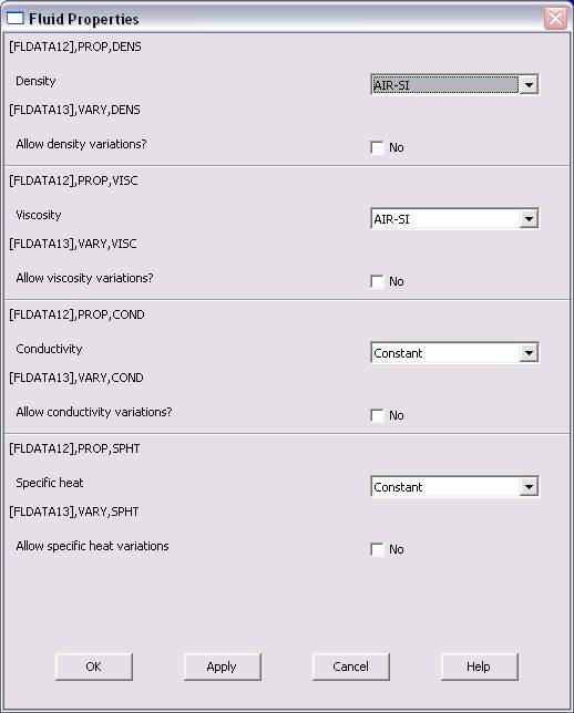
· Go to Preprocessor>Flotran Set Up>Fluid Properties.

· On the box, shown below, make sure the first two input fields read AIR-SI, and then click on OK. Another box will appear. Click OK to accept the default values.

· Now we’re ready to define the Material Properties

MATERIAL PROPERTIES

· Go to the ANSYS Main Menu

· Click Preprocessor>Material Props>Material Models. The following window will appear

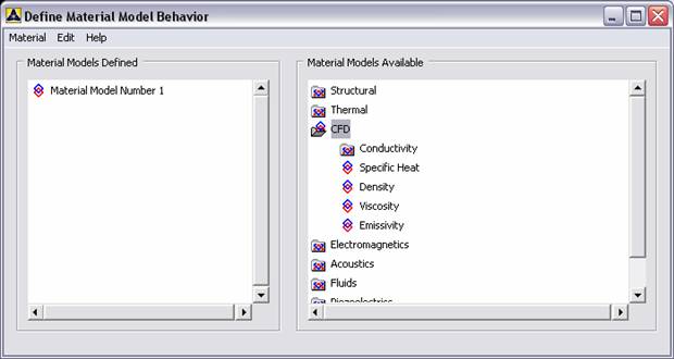
· As displayed, choose CFD>Density. The following window appears.

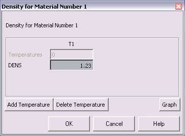
· Fill in 1.23 to set the density of Air. Click OK.

· Now choose CFD>Viscosity. The following window appears:

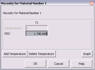
· Fill in 1.79e-5 to set the viscosity of Air. Click OK

· Now the Material 1 has the properties defined in the above table so the Material Models window may be closed.

MESHING:

DIVIDING THE CHANNEL INTO ELEMENTS:

· Go to Preprocessor>Meshing>Size Cntrls>ManualSize>Global>Size.

· In the window that comes up type 15 in the field for 'No. of element divisions'.

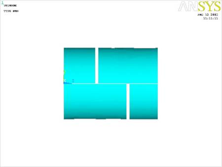
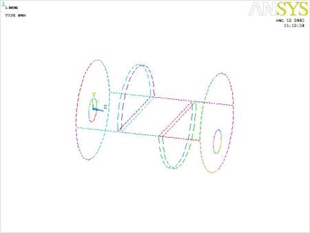
· Now go to Preprocessor>Meshing>Mesh>Volumes>Free. Click the muffler then Click OK. The mesh will look like the following.

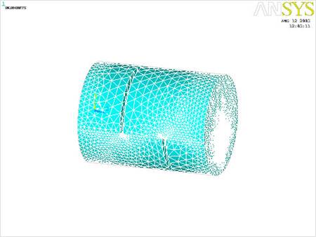
NOTE: The mountains are meshed safely inside the block. Do not be alarmed that you can not see them.

BOUNDARY CONDITIONS AND CONSTRAINTS

· Go to Preprocessor>Loads>Define Loads>Apply>Fluid CFD>Velocity>On Areas. Pick the inlet of the muffler and Click OK. The following window comes up.

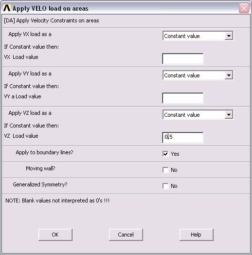
· Enter 0.5 in the VZ value field and click OK. The 0.5 corresponds to the velocity of 0.5 meters per second of air flowing into the muffler.

· Then, set the Velocity to ZERO along all of the sides of the cylinder forming the muffler. DO NOT FORGET the walls of the impedances though, this is very important because indeed, no air flows along the edges of those walls. This impeded flow is because of the “No Slip Condition” acting on all theoretical walls. (VX=VY=0 for all sides)

· Go to Main Menu>Preprocessor>Loads>Define Loads>Apply>Fluid CFD>Pressure DOF>On Areas. Pick the area defining the exit of the muffler and click OK.

· Enter 0 as the pressure value. (This sets the pressure as atmospheric allowing the air to pass over the car)

· Once all the Boundary Conditions have been applied, we can move on to solving the problem.

SOLUTION

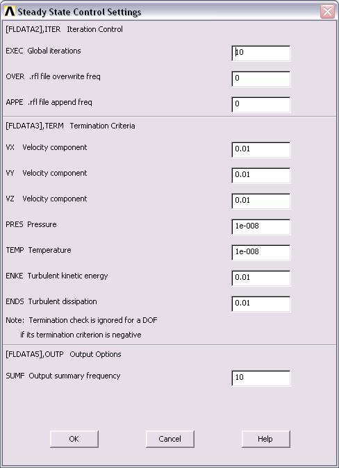
· Go to ANSYS Main Menu>Solution>Flotran Set Up>Execution Ctrl.

· The following window appears. Change the first input field value to 10, as shown. No other changes are needed. Click OK.

· Go to Solution>Run FLOTRAN.

· Wait for ANSYS to solve the problem.

· Click on OK and close the 'Information' window.

POST-PROCESSING

· Plotting the velocity distribution…

· Go to General Postproc>Read Results>Last Set.

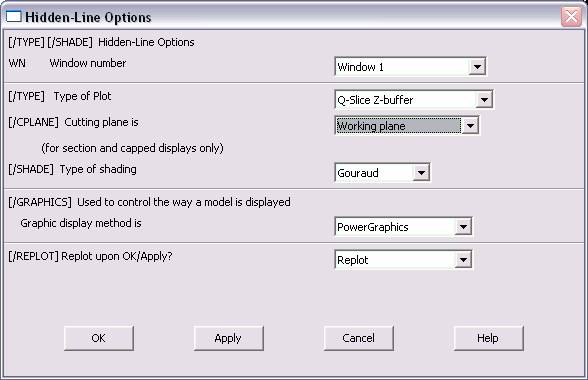
· Then, go to the ANSYS Main Menu (the Top Bar) and Click Plot>Volumes.

· After the volumes have been plotted, go to the ANSYS Main Menu>WorkPlane and select Display Working Plane. Now that the working plane is selected, go to ANSYS Main Menu>WorkPlane >Offset WP by Increments and rotate the working plane about the –Y axis such that it bisects the cylinder along is longest axis.

(NOTE: you can make sure it is properly positioned by selecting ANSYS Main Menu>PlotCntrls>Pan Zoom Rotate and changing the views to verify).

Once the plane is in line, select ANSYS Main Menu>PlotCntrls>Style…>Hidden Line Options.. a pop up window will now appear:

In this window change “Type of Plot” to Q-Slice Z-buffer, and “Cutting Plane is” to Working Plane and click OK. ANSYS will now display the results of the analysis with the working plane as the cutting plane.

· Then go to General Postproc>Plot Results>Contour Plot>Nodal Solution. The following window appears:

· Select DOF Solution and Velocity and Click OK.

The final solution now looks like this:

· Next go back to the ANSYS Main Menu>PlotCntrls>Style…>Hidden Line Options and change the values back to their original settings. (“Type of Plot” to Z-buffered, and “Cutting Plane is” to Normal to View)

· Go to Main Menu>General Postproc>Plot Results>Vector Plot>Predefined. The following window will appear:

· Select OK to accept the defaults. This will display the vector plot of the velocity gradient.

This is the final solution.