·
Check
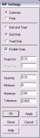
the Cartesian and Grid Only buttons
·
Enter
the values shown in the figure above.
·
Go to
the ANSYS Main Menu
·
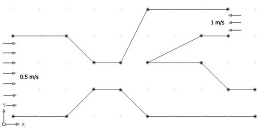
In this
problem we will model the pipe grid and then apply fluid flow to it.
·
Click
Preprocessor>-Modeling->
and create the pipe grid as shown below.
·
Hint:
You can use key points and then create the area
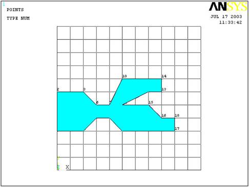
The modeling of the
problem is done.
ELEMENT PROPERTIES
SELECTING ELEMENT
TYPE:
·
Click
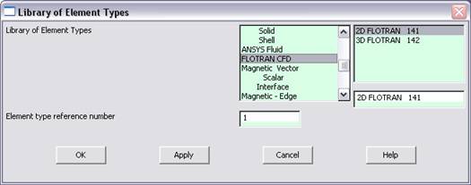
Preprocessor>Element Type>Add/Edit/Delete...
In the 'Element Types' window that opens click on Add... The
following window opens:
·
Type
1 in the Element type reference number.
·
Click
on Flotran CFD and select
2D Flotran 141. Click OK. Close
the 'Element types' window.
·
So now
we have selected Element type 1 to be a Flotran
element. The component will now be modeled using the principles of fluid
dynamics. This finishes the selection of element type.
DEFINE THE FLUID
PROPERTIES:
·
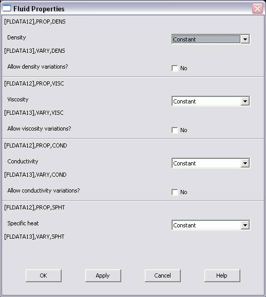
Go
to
Preprocessor>Flotran Set Up>Fluid
Properties.
·
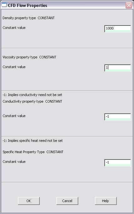
On the
box, shown below, make sure the first two input fields read Constant,
and then click on OK. Another box will appear. Fill in the
values as shown below, then click OK.
·
Now
we’re ready to define the Material Properties
MATERIAL PROPERTIES
·
Go to
the ANSYS Main Menu
·
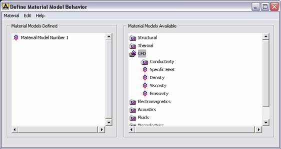
Click
Preprocessor>Material Props>Material Models.
The following window will appear
·
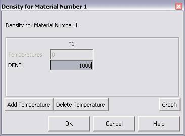
As
displayed, choose CFD>Density. The following window appears.
·
Fill in
1000 to set the density of Water. Click OK.
·
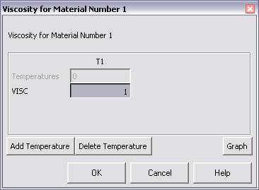
Now
choose CFD>Viscosity. The following window appears:
·
Fill in
1 to set the viscosity of Water. Click OK
·
Now the
Material 1 has the properties defined in the above table so the Material
Models window may be closed.
MESHING:
DIVIDING THE CHANNEL
INTO ELEMENTS:
·
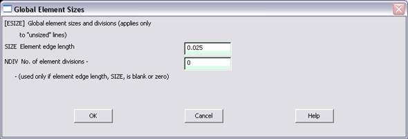
Go to
Preprocessor>Meshing>Size Cntrls>ManualSize>Global>Size.
In the window that comes up type 0.025 in the field for 'Element
edge length'.
·
Click
on OK. Now when you mesh the figure ANSYS will automatically create a
mesh, whose elements have a edge length of
0.025 m.
·
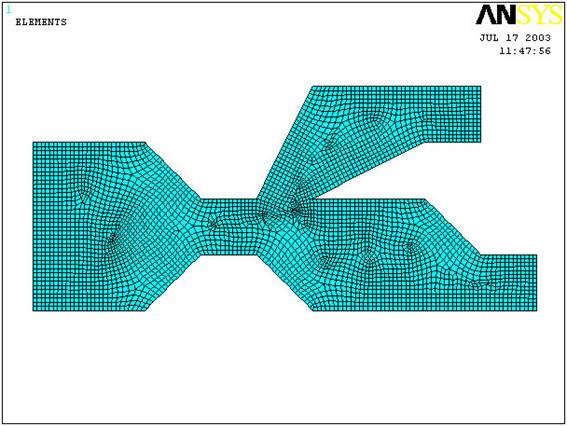
Now go
to
Preprocessor>Meshing>Mesh>Areas>Free.
Click Pick All. The mesh will look like the following.
BOUNDARY CONDITIONS AND
CONSTRAINTS
·
Go to
Preprocessor>Loads>Define
Loads>Apply>Fluid CFD>Velocity>On lines.
Pick the left edge of the block and Click OK. The following
window comes up.
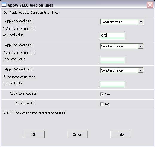
·
Enter
0.5 in the VX value field and click OK. The 0.5 corresponds to
the velocity of 0.5 meters per second of air flowing into the pipe grid.
·
Repeat
the above and set the velocity into the upper pipe as -1
meter/second. This is because the flow is traveling to the left, or the
negative direction.
·
Then,
set the Velocity to ZERO along all of the edges of the pipes.
This is because of the “No Slip Condition” (VX=VY=0 for all sides)
·
Go to
Main
Menu>Preprocessor>Loads>Define Loads>Apply>Fluid
CFD>Pressure DOF>On Lines.
Pick the bottom pipe outlet and click OK.
·
Once
all the Boundary Conditions have been applied, the pipe grid will look
like this:

·
Now the
Modeling of the problem is done.
SOLUTION
·
Go
to ANSYS
Main
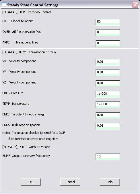
Menu>Solution>Flotran Set Up>Execution Ctrl.
·
The following window appears. Change the first input field value to
50, as shown. No other changes are needed. Click OK.
·
Go
to
Solution>Run FLOTRAN.
·
Wait for ANSYS to solve the problem.
·
Click on OK and close the 'Information' window.
POST-PROCESSING
·
Plotting the velocity distribution…
·
Go
to
General
Postproc>Read
Results>Last Set.
·
Then go to
General
Postproc>Plot
Results>Contour Plot>Nodal Solution.
The following window appears:
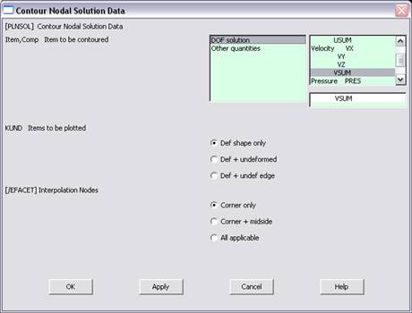
·
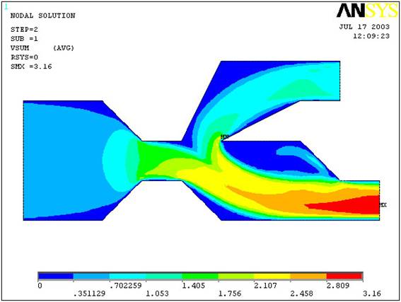
Select DOF Solution and Velocity VSUM and Click OK.
·
This is what the solution should look like:
·
Next, go to
Main
Menu>General Postproc>Plot Results>Vector
Plot>Predefined.
The following window will appear:
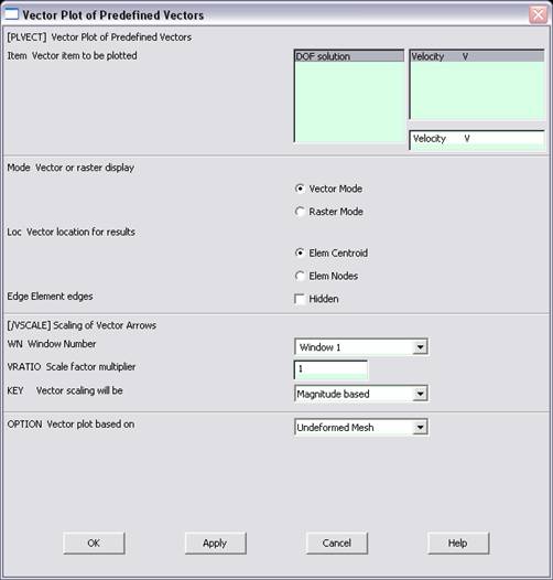
·
Select OK to accept the defaults. This will display the vector
plot of the velocity gradient.