Fluid #2: Flow
Around An Airfoil USING HEAT ANALOGY
Introduction:
In this example
you will model air flow over an airfoil.
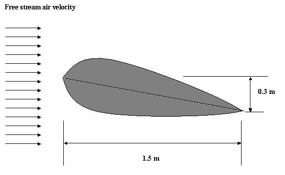
Physical Problem:
Compute
and plot the velocity distribution over the airfoil shown below.
Problem Description:
·
The
chord of the airfoil has dimensions and orientation as shown in the
figure.
·
The
flow velocity of air is 2m/s.
·
Objective:
To plot the velocity profile around the airfoil.
To graph the velocity distribution above and
below the airfoil.
·
You are
required to hand in print outs for the above.
·
Figure:
IMPORTANT:
Convert all
dimensions and forces into SI units.
Starting ANSYS:
·
Click
on ANSYS 6.1
in the programs menu.
·
Select
Interactive.
·
The
following menu comes up. Enter the working directory. All your files
will be stored in this directory. Also under
Use Default Memory Model make sure
the values 64 for Total
Workspace, and 32 for
Database are entered. To change these values unclick
Use Default Memory Model.
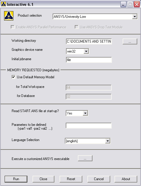
·
Click
RUN
MODELING THE STRUCTURE
·
Go to
the ANSYS Utility Menu
·
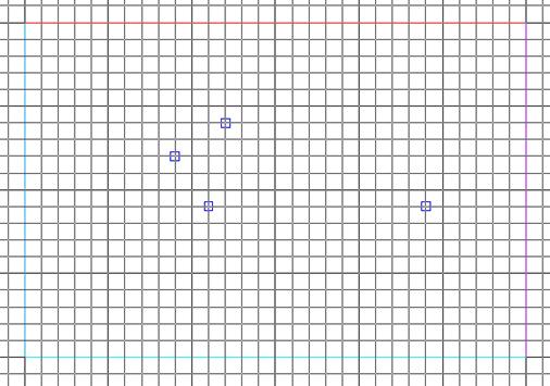
Click
Workplane>WP
Settings
·
The
following window will appear:
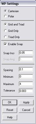
·
Check
the Cartesian and Grid Only buttons
·
Enter
the values shown in the figure above.
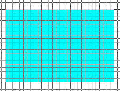
·
Go to
the ANSYS Main Menu.
·
Click
Preprocessor>-Modeling->
and create a rectangle of dimensions 3mX2m. The created rectangle should
look like the figure below:
·
Creating the airfoil.
·
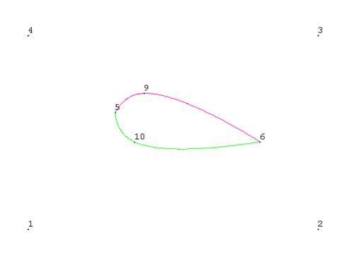
Go to
Main
Menu>Preprocessor>-Modeling->Create>Keypoints.
·
Create
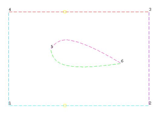
the keypoints as shown in the figure below:
·
Note
that I have only plotted the boundary lines of the rectangle created
before to make it easier to see the keypoints.
·
Go to
Main
Menu>Preprocessor>-Modeling->Create>-Lines->Splines
thru Keypoints
·
Create
two splines through the top three and the
bottom three splines. The figure should look
like the one below:
·
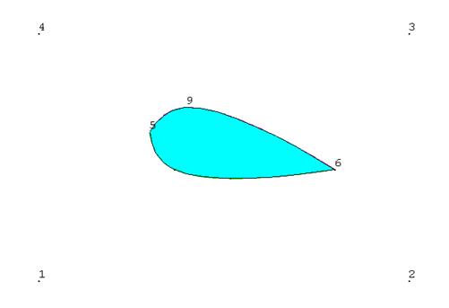
Now
create an area enclosed by the two splines.
Go to
Modeling>Create>Areas>Arbitrary>By Lines.
·
Pick
the two splines and click OK. The
model should look like the one below.
·
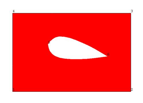
Now
subtract this airfoil area from the rectangle area. Go to
Postprocessor>Modeling>Operate>Booleans>Subtract>Areas
and then select the larger area, then the airfoil. The figure should
look like the following:
·
The
modeling of the problem is done.
ELEMENT PROPERTIES
SELECTING ELEMENT
TYPE:
·
Click
Preprocessor>Element Type>Add/Edit/Delete...
In the 'Element Types' window that opens click on Add... The
following window opens:
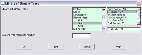
·
Type
1 in the Element type reference number.
·
Click
on Thermal Solid and select 8node. Click OK. Close
the 'Element types' window.
·
So now
we have selected Element type 1 to be a thermal solid 8node element. The
component will now be modeled with thermal solid 8node elements. This
finishes the selection of element type.
MATERIAL PROPERTIES
·
We will
model the fluid flow problem as a thermal conduction problem. The flow
corresponds to heat flux, pressure corresponds to temperature difference
and permeability corresponds to conductance.
·
Go to
the ANSYS Main Menu
·
Click
Preprocessor>Material Props>-Constant->Isotropic.
The following window will appear
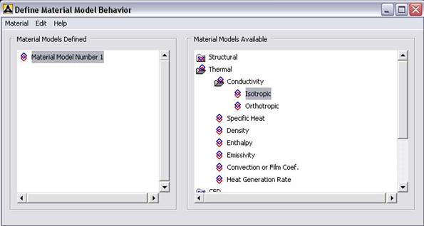
·
Enter
1 for the Material Property Number and click OK.
The following window will appear:
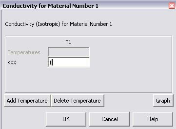
·
Fill in
1 for Thermal conductivity. Click OK.
·
Now
Material 1 has the properties defined in the above table. This
represents the material properties for the fluid in the channel.
MESHING:
·
DIVIDING THE CHANNEL INTO ELEMENTS:
·
Go to
Preprocessor>Meshing>Size Cntrls>ManualSize>Global>Size.
In the window that appears type 0.1 in the field for 'Element
edge length'.
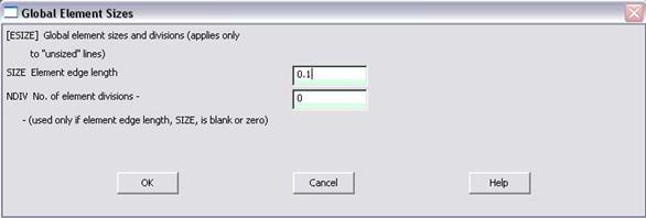
·
Click
on OK. Now when you mesh the figure ANSYS will automatically
create a mesh, whose elements have a edge
length of 0.1 m.
·
Now go
to
Preprocessor>-Meshing->Mesh>Areas>Free.
Click Pick All. The mesh should look like the following:

BOUNDARY CONDITIONS
AND CONSTRAINTS
·
Go to
Preprocessor>Loads>-Load->Apply>-Thermal->Heat
Flux>On lines.
Pick the left line of the rectangle. Click OK. The following
window will appear:
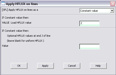
·
Enter
2 in the HFLUX value field and click OK.
the 2 corresponds to the inlet velocity of 2
m/s.
·
Repeat
the above for the right line of the rectangle. Remember this is
negative since it is leaving this side of the system, so include the
negative sign.
·
The
figure should look like the one below:

·
Now the
Modeling of the problem is done.
·
Go to
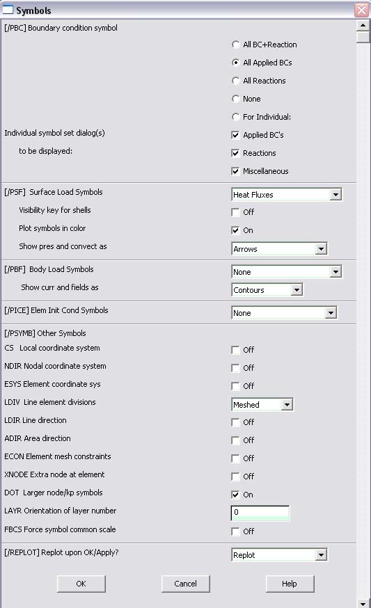
Utility Menu>PlotCtrls>Symbols.
The following window will appear:
·
Fill in
the values as shown and click OK. This sets up the arrow symbol
to denote the heat fluxes, which in turn represent the fluid velocity.
·
Now go
to the Utility Menu>Plot>Lines.
SOLUTION
·
Go to
ANSYS
Main Menu>Solution>-Analysis Type->New Analysis.
·
Select
"Steady State" and click on OK.
·
Go to
Solution>-Solve->Current LS.
·
Wait
for ANSYS to solve the problem.
·
Click
on OK and close the 'Information' window.
POST-PROCESSING
·
Plotting the velocity vectors
·
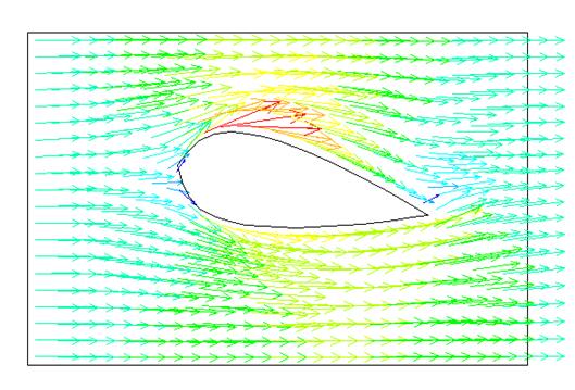
Now go
to
General
Postproc>Plot Results>-Vector
Plot->Predefined.
The following window will appear:
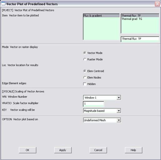
·
Enter
the values as shown and click OK. The plot of velocities will
look as follows.
·
To plot
the graph of variation of the velocity along the airfoil.
·
Go to
Utility
Menu>Plot>Areas.
·
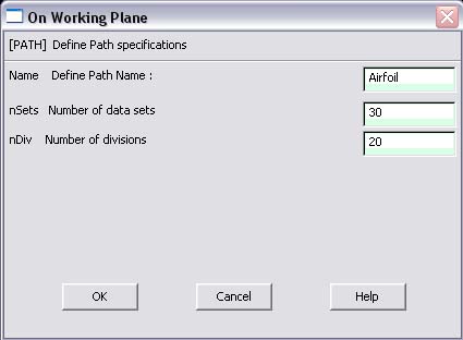
Go to
Main
Menu>General Postproc>Path Operations>Define
Path>On Working Plane
·
Pick
points at the ends of the elbow as shown. We will graph the velocity
distribution along the line joining these two points.
·
The
following window will appear:
·
Enter
the values as shown.
·
Now go
to
Main
Menu>General Postproc>Path Operations>Map
onto Path.
The following window will appear:

·
Now go
to
Main
Menu>General Postproc>Path Operations>-Plot
Path Items->On Graph.
The following window will appear. Select VELOCITY and click OK.

·
The
graph should look as follows:

s>Define Path>On Working Plane+