F2 - Heat Analogy

For educational purposes, we have included this tutorial to explain a different way to solve the fluid problem expressed in the Channel tutorial in the Fluids Section of the ANSYS tutorials. Notice the disparity in the individual solutions.

Fluid #1: Velocity analysis in fluid flow in a channel using HEAT ANALOGY

Introduction: In this example you will model fluid flow in a channel

Physical Problem: Compute and plot the velocity distribution within the elbow. Assume that the flow is uniform at both the inlet and the outlet sections and that the elbow has uniform depth.

Problem Description:

The channel has dimensions as shown in the figure

The flow velocity as the inlet is 10 cm/s

Use the continuity equation to compute the flow velocity at exit

Objective:

To plot the velocity profile in the channel

To plot the velocity profile across the elbow

You are required to hand in print outs for the above

Figure:

IMPORTANT: Convert all dimensions and forces into SI units

STARTING ANSYS

	Click on ANSYS 6.1 in the programs menu.
	Select Interactive.
	The following menu comes up. Enter the working directory. All your files will be stored in this directory. Also under Use Default Memory Model make sure the values 64 for Total Workspace, and 32 for Database are entered. To change these values unclick Use Default Memory Model

MODELING THE STRUCTURE

	Go to the ANSYS Utility Menu (the top bar)
	Click Workplane>WP Settings…

The following window comes up:

o Check the Cartesian and Grid Only buttons

o Enter the values shown in the figure above

· Go to the ANSYS Main Menu (on the left hand side of the screen) and click

Preprocessor>Modeling>Create>Keypoints>On Working Plane

Create keypoints corresponding to the vertices in the figure. The keypoints look like below.

Now create lines joining these key points.

	Modeling>Create>Lines>Lines>Straight line
	The model looks like the one below.

Now create fillets between lines L4-L5 and L1-L2.

	Modeling>Create>Lines>Lines>Line Fillet
	The fillet radius is 0.1m. The model looks like the following now.

Now make an area enclosed by these lines.

	Modeling>Create>Areas>Arbitrary>By Lines
	Select all the lines and click OK. The model looks like the following

The modeling of the problem is done.

ELEMENT PROPERTIES

SELECTING ELEMENT TYPE:

	Click Preprocessor>Element Type>Add/Edit/Delete...
	In the 'Element Types' window that opens click on Add... The following window opens.

	Type 1 in the Element type reference number.
	Click on Thermal Solid and select 8node. Click OK. Close the 'Element types' window.
	So now we have selected Element type 1 to be a thermal solid 8node element. The component will now be modeled with thermal solid 8node elements. This finishes the selection of element type.

MATERIAL PROPERTIES

We will model the fluid flow problem as a thermal conduction problem.

The flow corresponds to heat flux, pressure corresponds to temperature difference and permeability corresponds to conductance.

	Go to the ANSYS Main Menu
	Click Preprocessor>Material Props>Material Library>Material Models. The following window will appear

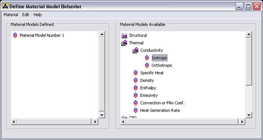
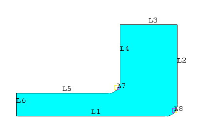
Double click Isotropic and when prompted with a window, enter 1 for the Kxx value. Now Exit Material Models.

Now the material 1 has the properties defined in the above table. This represents the material properties for the fluid in the channel.

MESHING:

DIVIDING THE CHANNEL INTO ELEMENTS:

Go to Preprocessor>Meshing>Size Cntrls>ManualSize>Areas>Picked Areas

Pick the area and then click ok. In the window that comes up type 0.05 in the field for 'Element edge length'.

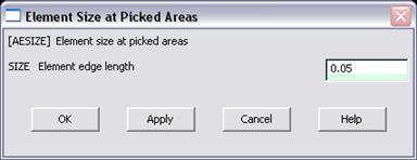
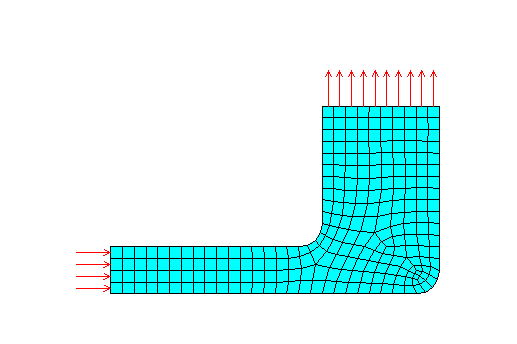
Click on OK. Now when you mesh the figure ANSYS will automatically create a mesh, whose elements have a edge length of 0.05 m.

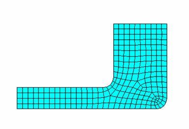
Now go to Preprocessor>Meshing>Mesh>Areas>Free. Click Pick All. The mesh will look like the following.

BOUNDARY CONDITIONS AND CONSTRAINTS

Go to Preprocessor>Loads>Load>Apply>Thermal>Heat Flux>On lines.

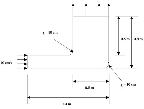
Pick the left line along the outer boundary (the inlet). Click OK. The following window comes up.

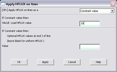
Enter 10 in the HFLUX value field and click OK. the 10 corresponds to the inlet velocity of 10cm/s.

Repeat the above for the outlet. First compute the outlet velocity using the continuity equation. Now apply this velocity at the outlet. Remember this is negative since it is leaving this system, so include the negative sign.

The figure looks something like below.

Now the Modeling of the problem is done.

Go to Utility Menu>PlotCtrls>Symbols. The following window comes up.

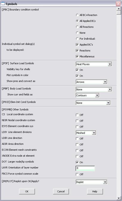
Fill in the values as shown and click OK. This sets up the arrow symbol to denote the heat fluxes, which in turn represent the fluid velocity.

Now go to the Utility Menu>Plot>Lines

SOLUTION

Go to ANSYS Main Menu>Solution>Analysis Type>New Analysis.

Select "Steady State" and click on OK.

Go to Solution>Solve>Current LS.

Wait for ANSYS to solve the problem.

Click on OK and close the 'Information' window.

POST-PROCESSING

Plotting the velocity vectors

Now go to General Postproc>Plot Results>Vector Plot>Predefined. The following window comes up.

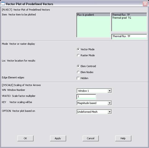
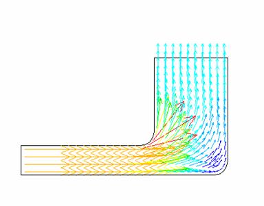
Enter the values as shown and click OK. The plot of velocities will look as follows.

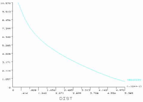
To plot the graph of variation of the velocity along the elbow.

Go to Utility Menu>Plot>Areas.

Go to Main Menu>General Postproc>Path Operations>Define Path>By Nodes

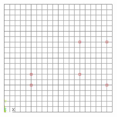
Pick points at the ends of the elbow as shown. We will graph the velocity distribution along the line joining these two points.

The following window comes up.

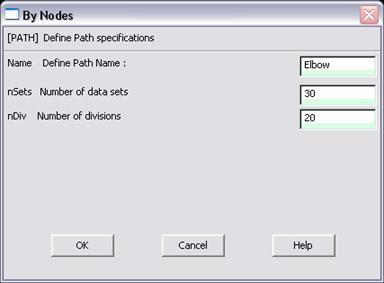
Enter the values as shown.

Now go to Main Menu>General Postproc>Path Operations>Map onto Path. The following window comes up.

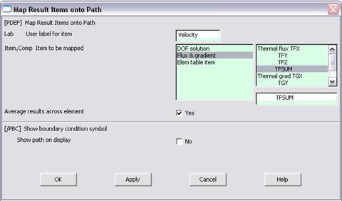
Now go to Main Menu>General Postproc>Path Operations>Plot Path Items>On Graph.

The following window comes up.

Select VELOCITY and click OK.

The graph will look as follows.

F2 - Heat Analogy - Channel