F2 Channel

Fluid #2: Velocity analysis of fluid flow in a channel USING FLOTRAN

Introduction: In this example you will model fluid flow in a channel

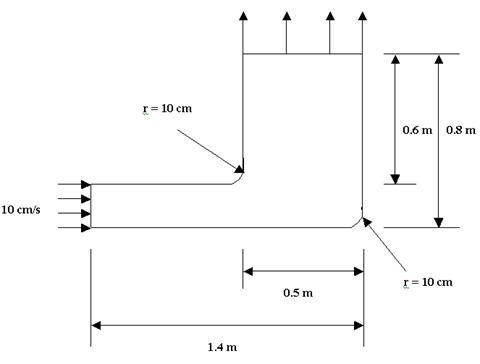
Physical Problem: Compute and plot the velocity distribution within the elbow. Assume that the flow is uniform at both the inlet and the outlet sections and that the elbow has uniform depth.

Problem Description:

The channel has dimensions as shown in the figure

The flow velocity as the inlet is 10 cm/s

Use the continuity equation to compute the flow velocity at exit

Objective:

To plot the velocity profile in the channel

To plot the velocity profile across the elbow

You are required to hand in print outs for the above

Figure:

IMPORTANT: Convert all dimensions and forces into SI units

STARTING ANSYS

	Click on ANSYS 6.1 in the programs menu.
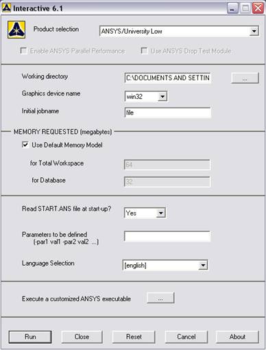
	Select Interactive.
	The following menu comes up. Enter the working directory. All your files will be stored in this directory. Also under Use Default Memory Model make sure the values 64 for Total Workspace, and 32 for Database are entered. To change these values unclick Use Default Memory Model

MODELING THE STRUCTURE

	Go to the ANSYS Utility Menu (the top bar)
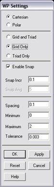
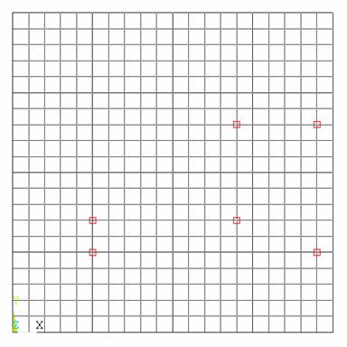
	Click Workplane>WP Settings…

The following window comes up:

o Check the Cartesian and Grid Only buttons

o Enter the values shown in the figure above

· Go to the ANSYS Main Menu (on the left hand side of the screen) and click

Preprocessor>Modeling>Create>Keypoints>On Working Plane

Create keypoints corresponding to the vertices in the figure. The keypoints look like below.

Now create lines joining these key points.

	Modeling>Create>Lines>Lines>Straight line
	The model looks like the one below.

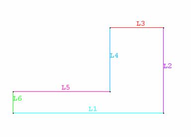
Now create fillets between lines L4-L5 and L1-L2.

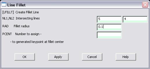
Click Modeling>Create>Lines>Line Fillet. A pop-up window will now appear. Select lines 4 and 5. Click OK. The following window will appear:

	This window assigns the fillet radius. Set this value to 0.1 m.
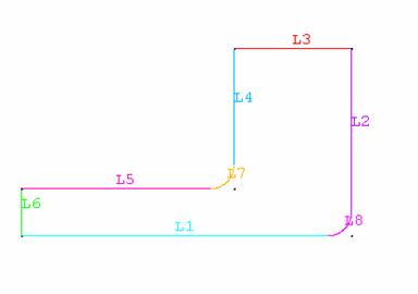
	Repeat this process of filleting for Lines 1 and 2.
	The model should look like this now:

Now make an area enclosed by these lines.

	Modeling>Create>Areas>Arbitrary>By Lines
	Select all the lines and click OK. The model looks like the following

The modeling of the problem is done.

ELEMENT PROPERTIES

SELECTING ELEMENT TYPE:

· Click Preprocessor>Element Type>Add/Edit/Delete... In the 'Element Types' window that opens click on Add... The following window opens.

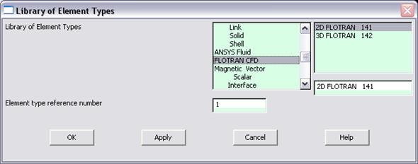
· Type 1 in the Element type reference number.

· Click on Flotran CFD and select 2D Flotran 141. Click OK. Close the Element types window.

· So now we have selected Element type 1 to be solved using Flotran, the computational fluid dynamics portion of ANSYS. This finishes the selection of element type.

DEFINE THE FLUID PROPERTIES:

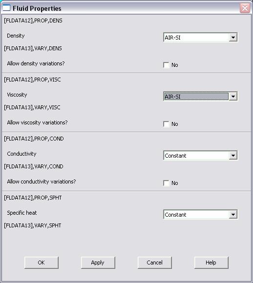
· Go to Preprocessor>Flotran Set Up>Fluid Properties.

· On the box, shown below, set the first two input fields as Air-SI, and then click on OK. Another box will appear. Accept the default values by clicking OK.

· Now we’re ready to define the Material Properties

MATERIAL PROPERTIES

	We will model the fluid flow problem as a thermal conduction problem. The flow corresponds to heat flux, pressure corresponds to temperature difference and permeability corresponds to conductance.
	Go to the ANSYS Main Menu
	Click Preprocessor>Material Props>Material Models. The following window will appear

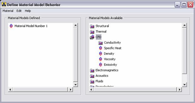
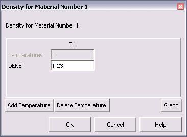
As displayed, choose CFD>Density. The following window appears.

	Fill in 1.23 to set the density of Air. Click OK.
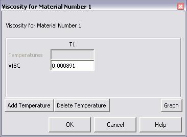
	Now choose CFD>Viscosity. The following window appears:

Now the Material 1 has the properties defined in the above table so the Material Models window may be closed.

MESHING:

DIVIDING THE CHANNEL INTO ELEMENTS:

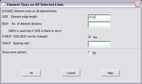
	Go to Preprocessor>Meshing>Size Cntrls>ManualSize>Lines>All Lines.
	In the window that comes up type 0.01 in the field for 'Element edge length'.

	Now Click OK.
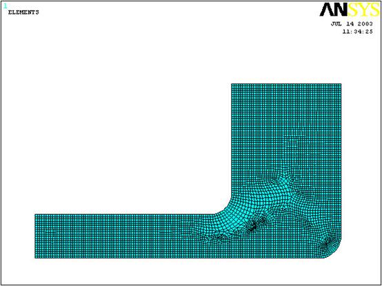
	Now go to Preprocessor>Meshing>Mesh>Areas>Free. Click the area and the OK. The mesh will look like the following.

BOUNDARY CONDITIONS AND CONSTRAINTS

Go to Preprocessor>Loads>Define Loads>Apply>Fluid CFD>Velocity>On lines. Pick the left edge of the outer block and Click OK. The following window comes up.

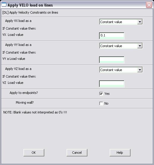
	Enter 0.1 in the VX value field and click OK. The 0.1 corresponds to the velocity of 0.1 meter per second of air flowing from the left side.
	Repeat the above and set the Velocity to ZERO for the air along all of the edges of the pipe. (VX=VY=0 for all sides)
	Once they have been applied, the pipe will look like this:

· Go to Main Menu>Preprocessor>Loads>Define Loads>Apply>Fluid CFD>Pressure DOF>On Lines.

· Pick the outlet line. (The horizontal line at the top of the area) Click OK.

· Enter 0 for the Pressure value.

· Now the Modeling of the problem is done.

SOLUTION

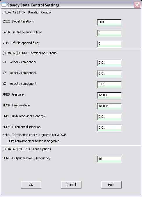
Go to ANSYS Main Menu>Solution>Flotran Set Up>Execution Ctrl.

· The following window appears. Change the first input field value to 300, as shown. No other changes are needed. Click OK.

	Go to Solution>Run FLOTRAN.
	Wait for ANSYS to solve the problem.
	Click on OK and close the 'Information' window.

POST-PROCESSING

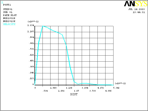
	Plotting the velocity distribution…
	Go to General Postproc>Read Results>Last Set.
	Then go to General Postproc>Plot Results>Contour Plot>Nodal Solution. The following window appears:

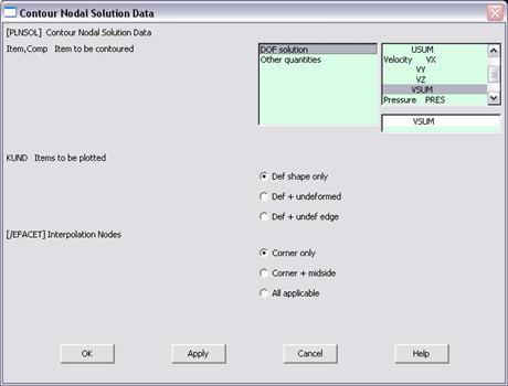
· Select DOF Solution and Velocity VSUM and Click OK.

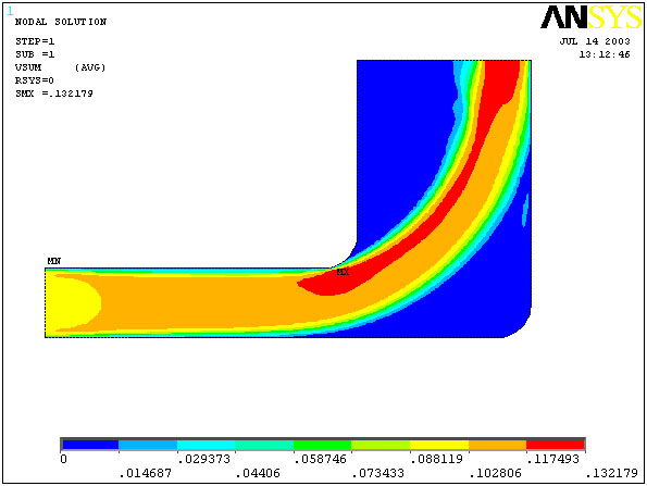
· This is what the solution should look like:

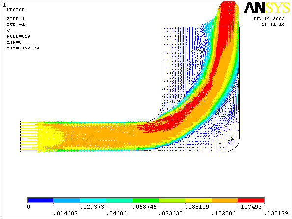
· Next, go to Main Menu>General Postproc>Plot Results>Vector Plot>Predefined. The following window will appear:

· Select OK to accept the defaults. This will display the vector plot to compare to the solution of the same tutorial solved using the Heat Flux analogy. Note: This analysis is FAR more precise as shown by the following solution:

· Go to Main Menu>General Postproc>Path Operations>Define Path>By Nodes

· Pick points at the ends of the elbow as shown. We will graph the velocity distribution along the line joining these two points.

· The following window comes up.

· Enter the values as shown.

· Now go to Main Menu>General Postproc>Path Operations>Map onto Path. The following window comes up.

· Now go to Main Menu>General Postproc>Path Operations>Plot Path Items>On Graph.

· The following window comes up.

· Select VELOCITY and click OK.

· The graph will look as follows: