F1 Airfoil

Fluid #1: Flow Around An Airfoil USING FLOTRAN

Introduction: In this example you will model air flow over an airfoil.

Physical Problem: Compute and plot the velocity distribution over the airfoil shown below.

Problem Description:

· The chord of the airfoil has dimensions and orientation as shown in the figure.

· The flow velocity of air is 2m/s.

· Objective:

To plot the velocity profile around the airfoil.

To graph the velocity distribution above and below the airfoil.

· You are required to hand in print outs for the above.

· Figure:

IMPORTANT: Convert all dimensions and forces into SI units.

Starting ANSYS:

· Click on ANSYS 6.1 in the programs menu.

· Select Interactive.

· The following menu comes up. Enter the working directory. All your files will be stored in this directory. Also under Use Default Memory Model make sure the values 64 for Total Workspace, and 32 for Database are entered. To change these values unclick Use Default Memory Model.

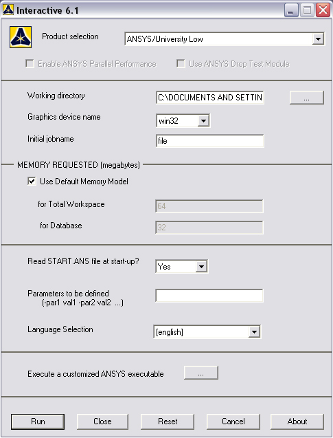
· Click RUN

MODELING THE STRUCTURE

· Go to the ANSYS Utility Menu

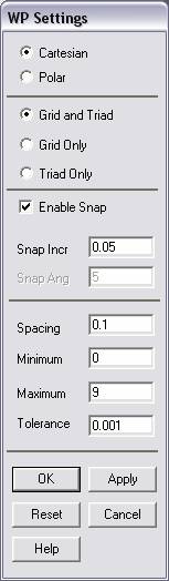
· Click Workplane>WP Settings

· The following window will appear:

· Check the Cartesian and Grid Only buttons

· Enter the values shown in the figure above.

· Go to the ANSYS Main Menu.

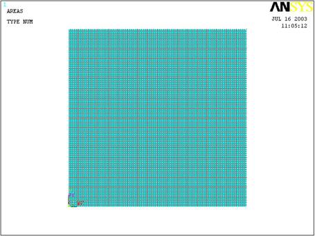
· Click Preprocessor>-Modeling-> and create a rectangle of dimensions 8mX8m. The created rectangle should look like the figure below:

· Creating the airfoil.

· Go to Main Menu>Preprocessor>-Modeling->Create>Keypoints>On Working Plane.

· Create the keypoints as shown in the figure below:

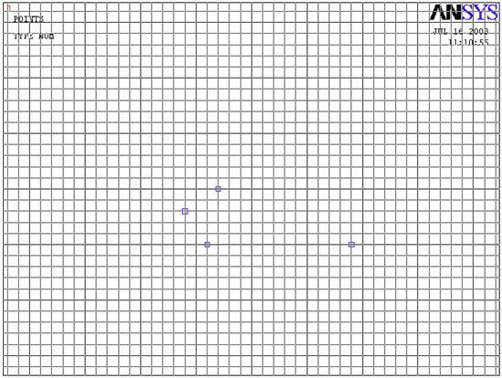
· Note that I have only plotted the boundary lines of the rectangle created before to make it easier to see the keypoints.

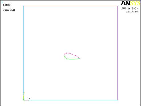
· Go to Main Menu>Preprocessor>-Modeling->Create>-Lines->Splines thru Keypoints

· Create two splines through the top three and the bottom three splines. The figure should look like the one below:

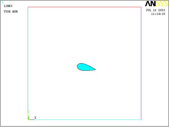
· Now create an area enclosed by the two splines. Go to Modeling>Create>Areas>Arbitrary>By Lines.

· Pick the two splines and click OK. The model should look like the one below.

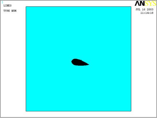
· Now subtract this airfoil area from the rectangle area. Go to Postprocessor>Modeling>Operate>Booleans>Subtract>Areas and then select the larger area, then the airfoil. The figure should look like the following:

· The modeling of the problem is done.

ELEMENT PROPERTIES

SELECTING ELEMENT TYPE:

· Click Preprocessor>Element Type>Add/Edit/Delete... In the 'Element Types' window that opens click on Add... The following window opens:

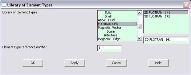
· Type 1 in the Element type reference number.

· Click on Flotran CFD and select 2D Flotran 141. Click OK. Close the 'Element types' window.

· So now we have selected Element type 1 to be a Flotran element. The component will now be modeled using the principles of fluid dynamics. This finishes the selection of element type.

DEFINE THE FLUID PROPERTIES:

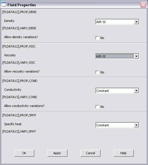
· Go to Preprocessor>Flotran Set Up>Fluid Properties.

· On the box, shown below, set the first two input fields as Air-SI, and then click on OK. Another box will appear. Accept the default values by clicking OK.

· Now we’re ready to define the Material Properties

MATERIAL PROPERTIES

	Go to the ANSYS Main Menu
	Click Preprocessor>Material Props>Material Models. The following window will appear

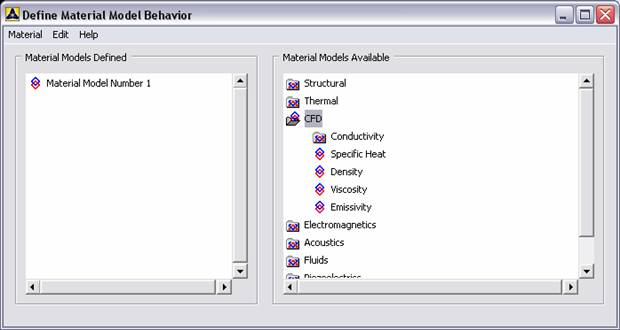
As displayed, choose CFD>Density. The following window appears.

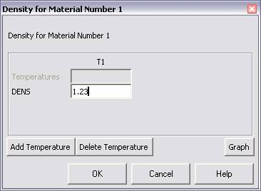
	Fill in 1.23 to set the density of Air. Click OK.
	Now choose CFD>Viscosity. The following window appears:

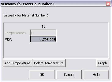
Now the Material 1 has the properties defined in the above table so the Material Models window may be closed.

MESHING:

DIVIDING THE AREA INTO ELEMENTS:

	Go to Preprocessor>Meshing>Size Cntrls>ManualSize>Lines>Picked Lines.
	Now choose the lines that form the airfoil in the center of the area. (Zooming In is most likely necessary. Do this by clicking in the ANSYS Utility Menu Plot Controls>Pan Zoom Rotate and then manipulating the block accordingly.)
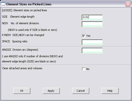
	In the window that comes up type 0.01 in the field for 'Element edge length'.

	Now Click OK. This step is such that more elements are set on the airfoil than on the edges of the larger area so that the analysis of the airfoil is more refined than the analysis of the area far away from the plate.
	Now, go to Preprocessor>Meshing>Size Cntrls>ManualSize>Lines>Picked Lines and pick the lines forming the outer area. This time, enter 0.2 as the Element edge length in the window that appears. Now when you mesh the figure ANSYS will automatically create a mesh that varies in detail from the plate to the edge of the outer block.
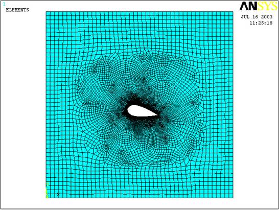
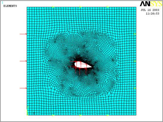
	Now go to Preprocessor>Meshing>Mesh>Areas>Free. Click the area and the OK. The mesh will look like the following.

BOUNDARY CONDITIONS AND CONSTRAINTS

Go to Preprocessor>Loads>Define Loads>Apply>Fluid CFD>Velocity>On lines. Pick the left edge block and Click OK. The following window comes up.

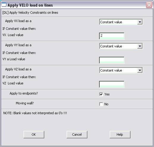
	Enter 2 in the VX value field and click OK. The 2 corresponds to the velocity of 2 meters per second of air flowing from the left side.
	Repeat the above and set the Velocity to ZERO for the air along all of the edges of the airfoil. (VX=VY=0 for all sides)
	Go to Main Menu>Preprocessor>Loads>Define Loads>Apply>Fluid CFD>Pressure DOF>On Lines. Pick the top, bottom, and right side of the block and click OK.
	Once all the Boundary Conditions have been applied, the airfoil will look like this:

· Now the Modeling of the problem is done.

SOLUTION

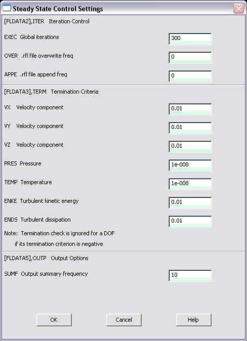
Go to ANSYS Main Menu>Solution>Flotran Set Up>Execution Ctrl.

· The following window appears. Change the first input field value to 300, as shown. No other changes are needed. Click OK.

	Go to Solution>Run FLOTRAN.
	Wait for ANSYS to solve the problem.
	Click on OK and close the 'Information' window.

POST-PROCESSING

	Plotting the velocity distribution…
	Go to General Postproc>Read Results>Last Set.
	Then go to General Postproc>Plot Results>Contour Plot>Nodal Solution. The following window appears:

· Select DOF Solution and Velocity VSUM and Click OK.

· This is what the solution should look like:

· Next, go to Main Menu>General Postproc>Plot Results>Vector Plot>Predefined. The following window will appear:

· Select OK to accept the defaults. This will display the vector plot to compare to the solution of the same tutorial solved using the Heat Flux analogy. Note: This analysis is FAR more precise as shown by the following solution:

· Go to Main Menu>General Postproc>Path Operations>Define Path>By Nodes

· Pick points at the ends of the elbow as shown. We will graph the velocity distribution along the line joining these two points.

· The following window comes up.

· Enter the values as shown.

· Now go to Main Menu>General Postproc>Path Operations>Map onto Path. The following window comes up.

· Now go to Main Menu>General Postproc>Path Operations>Plot Path Items>On Graph.

· The following window comes up.

· Select VELOCITY and click OK.

The graph will look as follows: