Overview
In this project, we will leverage deep neural networks to extract high level features from different images. Based on these extracted high-level features,
we use gradient-based optimization to "style transfer"
an image so that it matches target content image in the content space, and also matches target style image in the style space.
Neural Style Transfer Preview (From Course Assignment webpage)
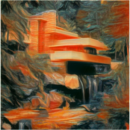
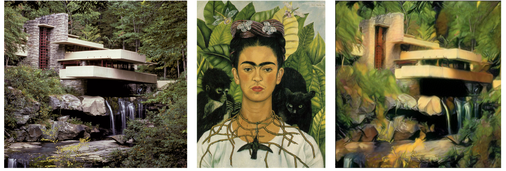 "Stylized" fallingwater
|
Part 1 Content Reconstruction
Using feature map from different layer as content metric
To measure the similarity of two images in terms of content, we need a representation of image in the content space.
Here we use a VGG-19 net pretrained on ImageNet to serve as feature extractor. Concretely, we use feature map from a
specific layer in the deep network as the content representation of image. As shown below, I compared the effect of using
different layers' feature map as content space. In general, using shallow layer as content loss will not result in large difference.
For instance, the reconstruction result from Conv1 and Conv3 is very close to the original image. We can observe more differences in results from
Conv4, Conv5, where the lighting of the image and contrastness has changed and also more noise are involved in the images. (For the rest experiments,
I use Conv4 as content loss layer)
 Original figure, JOJO
|
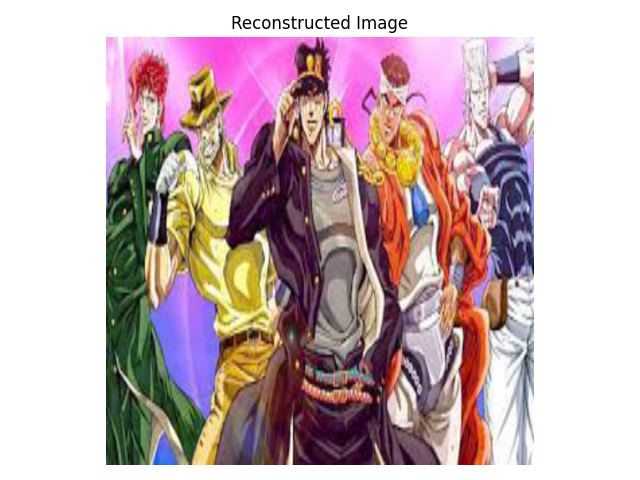 Using Conv1 as content loss layer
|
 Using Conv3 as content loss layer
|
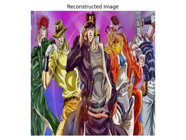 Using Conv4 as content loss layer
|
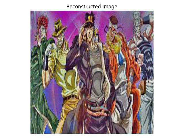 Using Conv5 as content loss layer
|
Optimization with random noise input
To test the sensitivity of this optimization scheme to initialization, I ran the optimization initialized with two randomly sampled noise. Qualitatively, there is no observable
difference between two results. The loss of image 1 is: 0.138228, and the loss of image 2 is: 0.138737, which are very close to each other.
Original figure, JOJO
|
 Optimization image 1
|
 Optimization image 2
|
Part 2 Texture Synthesis
To measure the similarity of images in the style space, similar to content loss implementation, we first extract high-level features of images using pretrained deep networks. Instead
of directly compare the distance of feature map vector, we use gram matrix to measure the style of an image, which is defined as:
$$G = f^L (f^L)^T$$
where \(f^L\) is a matrix with size \((N, K, H*W)\) which is formed by all the feature maps \(f_k\) at \(L\)-th layer of the network.
Using different layer to measure the style loss
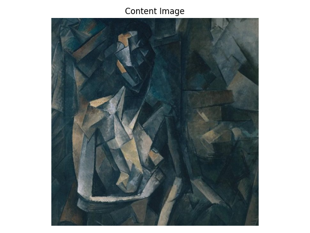 Original figure, Picasso
|
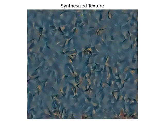
 Using Conv1, Conv2, Conv3, Conv4, Conv5 as loss layer
|
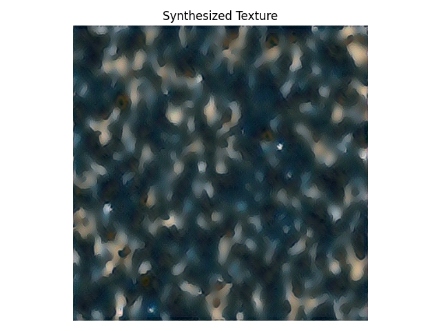 Using Conv1, Conv2 as loss layer
|
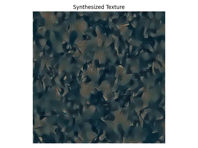
 Using Conv4, Conv5 as loss layer
|
From above results, we can see that from shallow layers (Conv1, Conv2), we will get more blurry images, while from deep layers (Conv4, Conv5), we will get sharper images.
In the rest experiments, I use Conv1, Conv2, Conv3, Conv4, Conv5 as style loss layers.
Optimization with random noise input
To test the sensitivity of this optimization scheme to initialization, I ran the optimization initialized with two randomly sampled noise. Qualitatively, we can see that for style loss
optimization, the result is much more sensitive to the initialization. Two optimization results with different random initialization looks quite different. The final loss of image 1 is
0.642954, for image2 it is 0.659186.
Original figure, Picasso
|
Optimization image 1
|
 Optimization image 2
|
Part 3 Style Transfer
To create an image that can both preserve the content of content image while having similar style with style image, the weights of different loss function need to be carefully tuned.
For Style loss, we first need to normalize the gram matrix. This can be achieved via dividing
the gram matrix by \(K*H*W\), where K is the channel numbers of feature map and H,W denotes height and width of feature map.
For the weight of loss function, empirically the weight for style loss should be larger than weight for content loss with 4~6 order of magnitude. I shown the results of using different
weight below. In general, 1e6 to 1e5 is a good weight to use (i.e. \(\lambda_{style}=10^6, \lambda_{content}=1\)). To make the stylized image more close to style target, we can
tweak the weight for style loss larger, but larger style weights will also make image lose some content information from content image.
Different loss hyperparameters
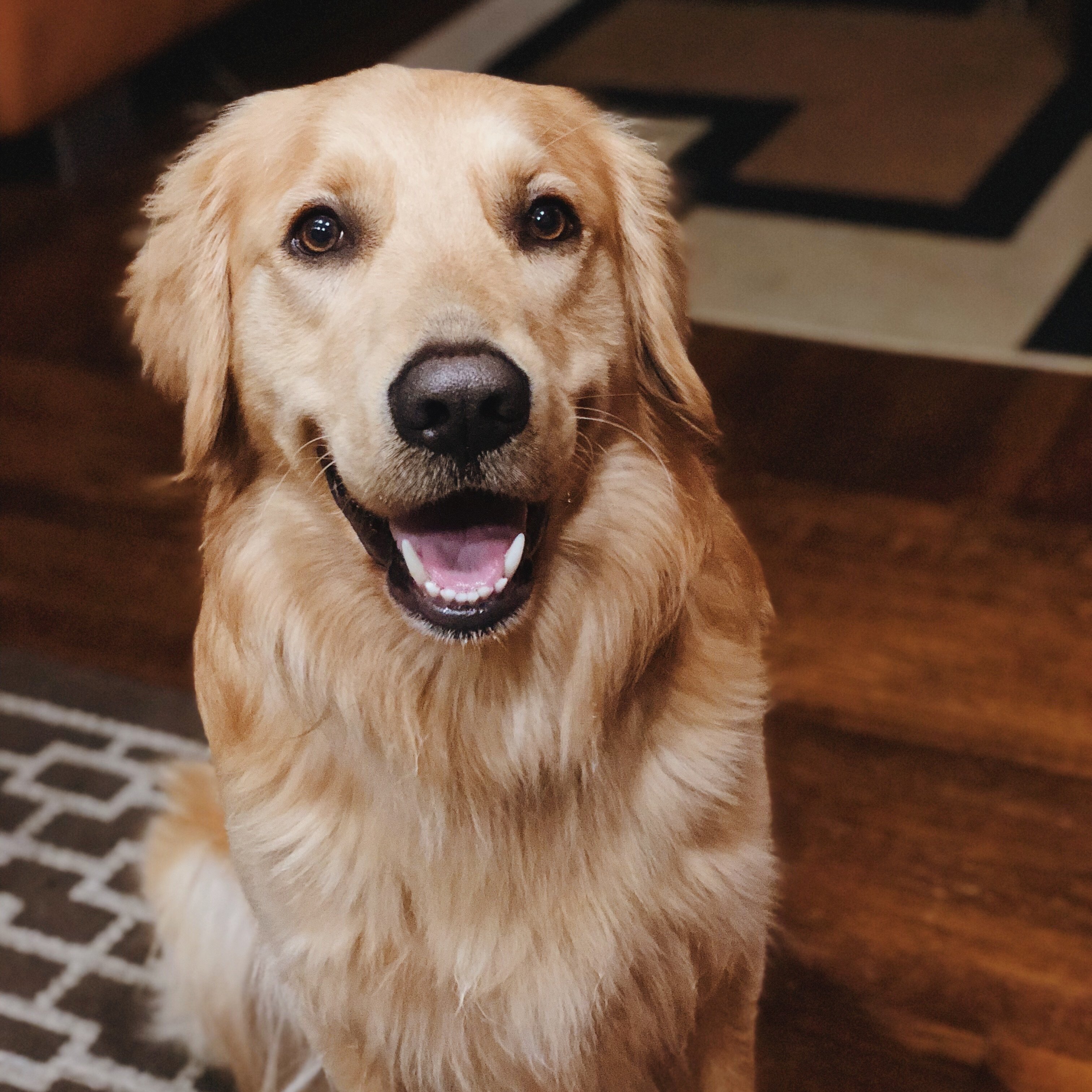 Content image, Wally
|
 Style image, Picasso
|
 \(\lambda_{style}=10^4, \lambda_{content}=1\) (Image quality is low)
|
 \(\lambda_{style}=10^6, \lambda_{content}=1\)
|
 \(\lambda_{style}=10^7, \lambda_{content}=1\)
|
 \(\lambda_{style}=10^8, \lambda_{content}=1\) (Content looks not natural)
|
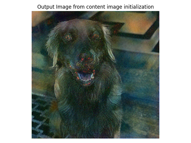
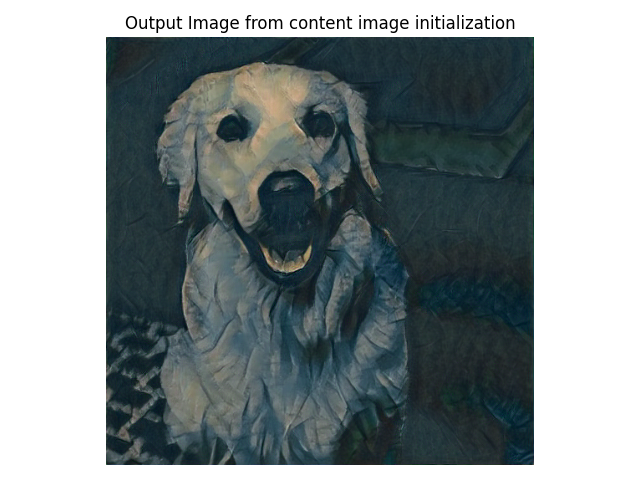
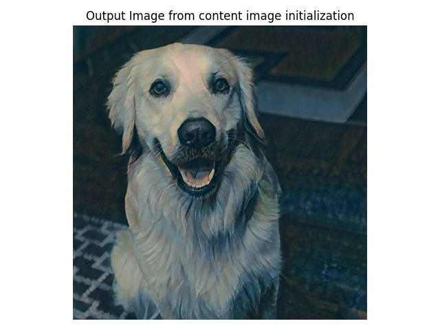
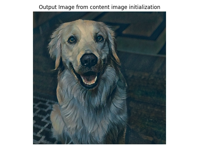
Comparison of using different initialization
From below, we can see that for random initialization, it took much more iterations to generate qualitative reasonable results (random initialization took 1000
iterations to get perceptually good result, but is still not as good as result using content image as initialization),
thus using content image as initialization is much more efficient.
 Use content image as initialization, after 300 iterations
|
 Use content image as initialization, after 500 iterations
|
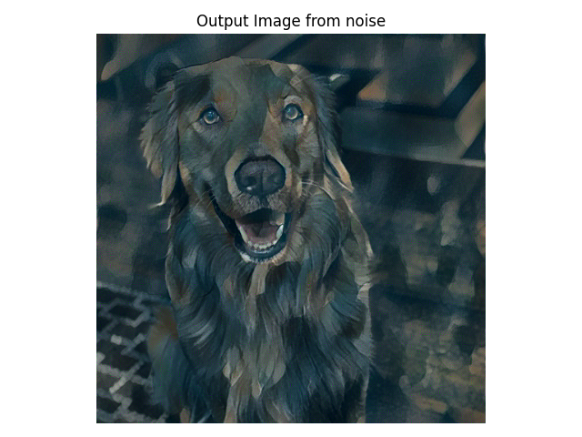 Use random noise as initialization, after 500 iterations
|
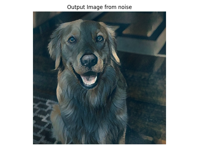 Use random noise as initialization, after 1000 iterations
|
Gallery
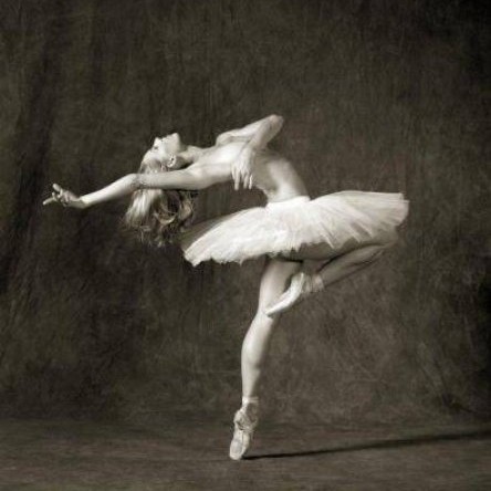 Content image, dancing
|
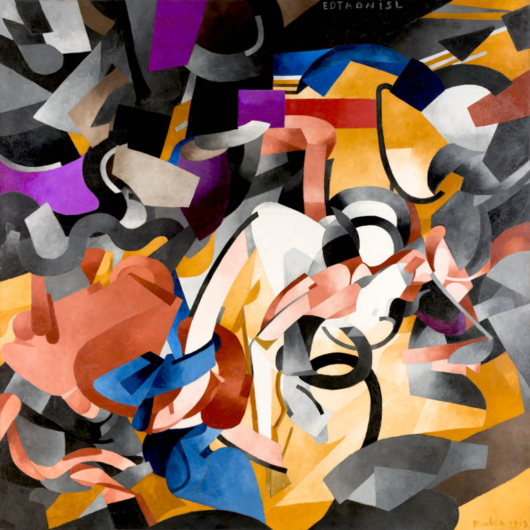 Style image, edtaonisl
|
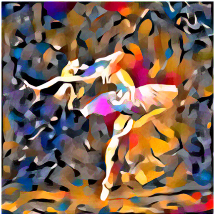 Stylize image
|
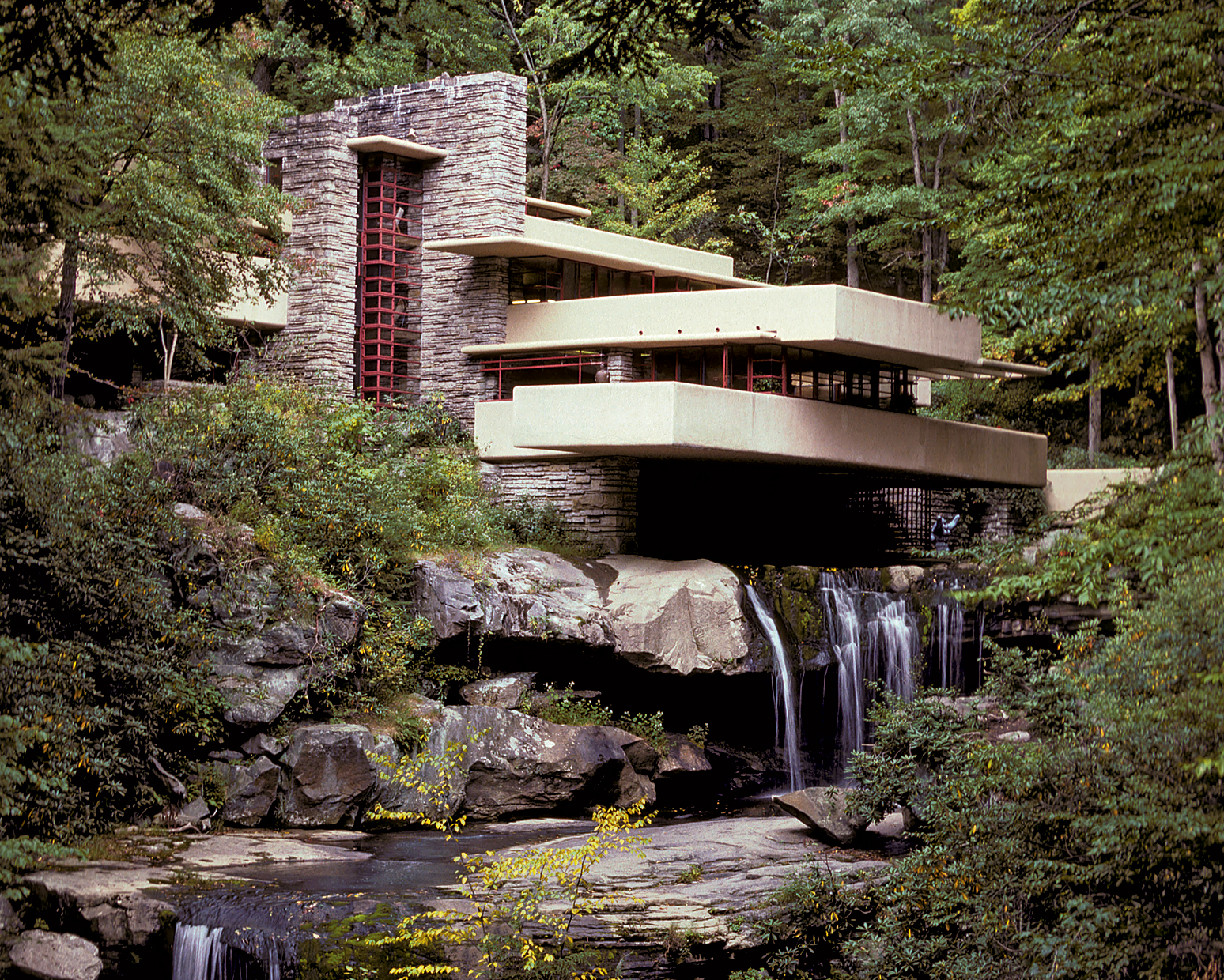 Content image, fallingwater
|
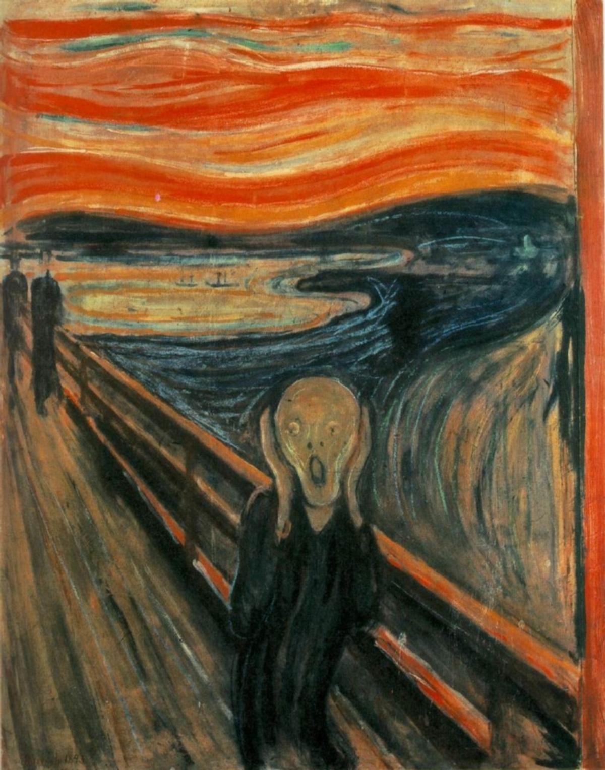 Style image, the scream
|
 Stylize image
|
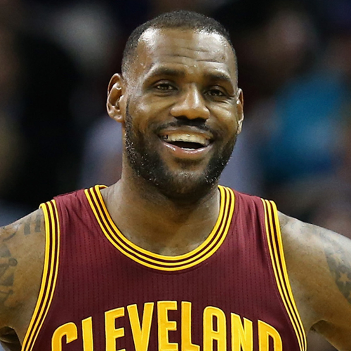 Content image, NBA star Lebron James
|
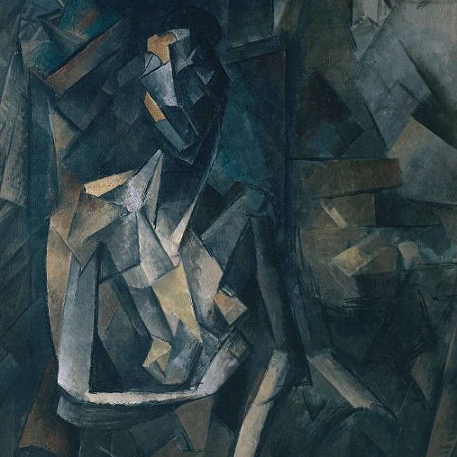 Style image, picasso
|
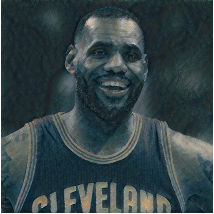 Stylize image
|
Bells and Whistles
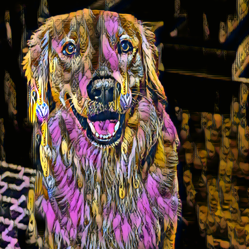
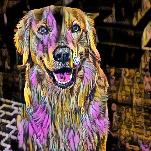
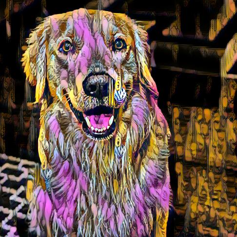
1. Stylized Grumpy Cat
 Content image, Grumpy cat B
|
 Style image, starry night
|
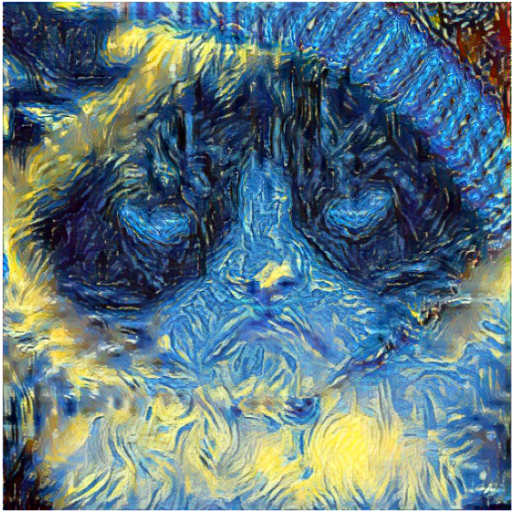 Stylize image, "starry cat"
|
 Content image, Grumpy cat A
|
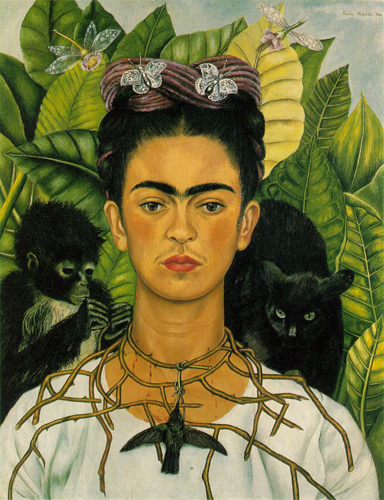 Style image, frida kahlo
|
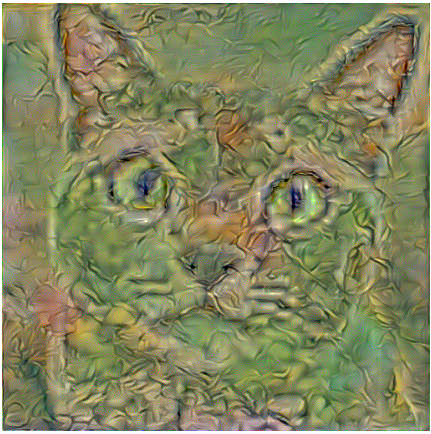 Stylize image, frida kahlo cat
|
2. Perceptual Losses for Real-Time Style Transfer and Super-Resolution
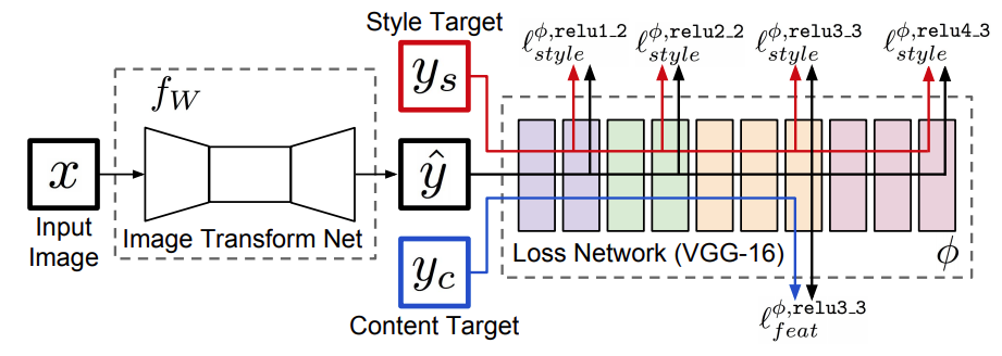 Framework in Perceptual Losses for Real-Time Style Transfer and Super-Resolution[1]
Slightly different from our assignment, in [1], instead of directly optimizing pixels, a feedforward network is used to generate images. Hence, it manipulates image in the weight
space (weights of the feed forward network). In this algorithm, the style image is fixed, which means for each style image, we will train a corresponding feed forward network. The
advantage of this method is that, we can pretrain a lot of different networks based on different style images and then in the inference stage we can stylize content image without any
iterative optimization which accelerates the style transfer speed.
The loss function is similar to the ones used in our assignment, but in the original paper it used vgg16 instead of vgg19. I implemented
the feed forward network (termed as Image Transform Net in the paper) with similar structure to one used in HW3. (3 convolutional layers, 5 residual blocks and 3 upsampling layers, here instead
of using transposed convolution, I use nearest interpolation + convolution to upsample the image, as this is reported to improve the overall performance).
According to the original paper, here I use MSCOCO (2014 training data) as the training dataset. The network is trained with 40k iterations and a batch size of 4, this process takes roughly 2 hours on GTX 1080Ti.
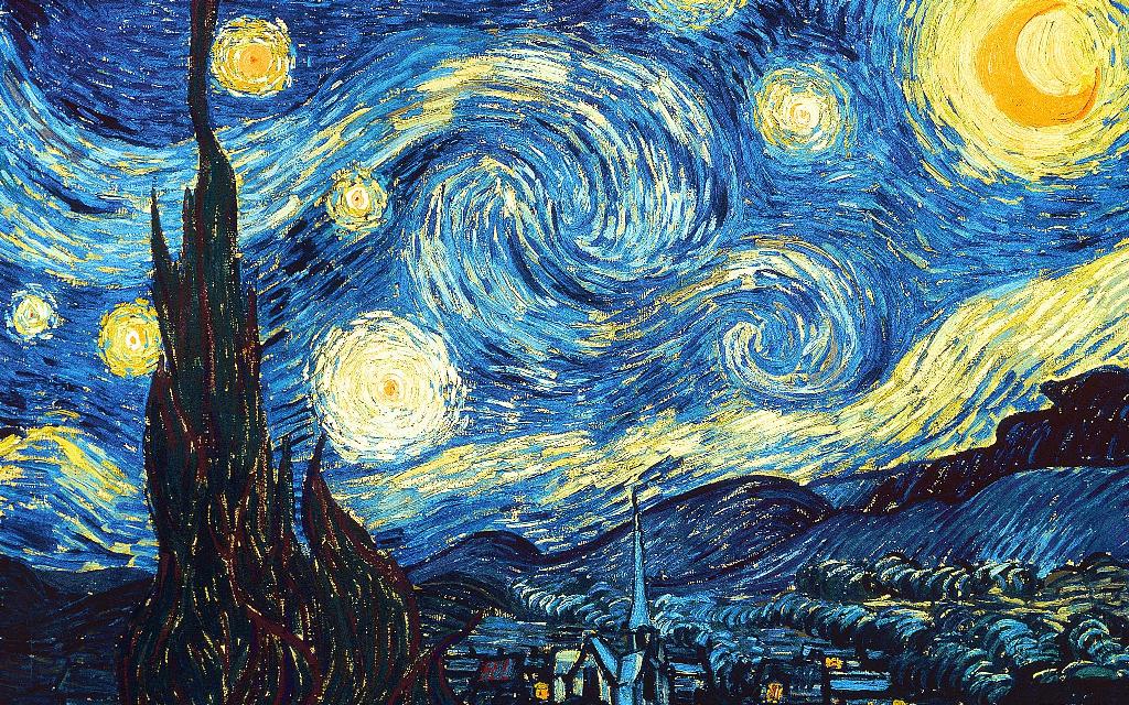 Style image, Starry night
|
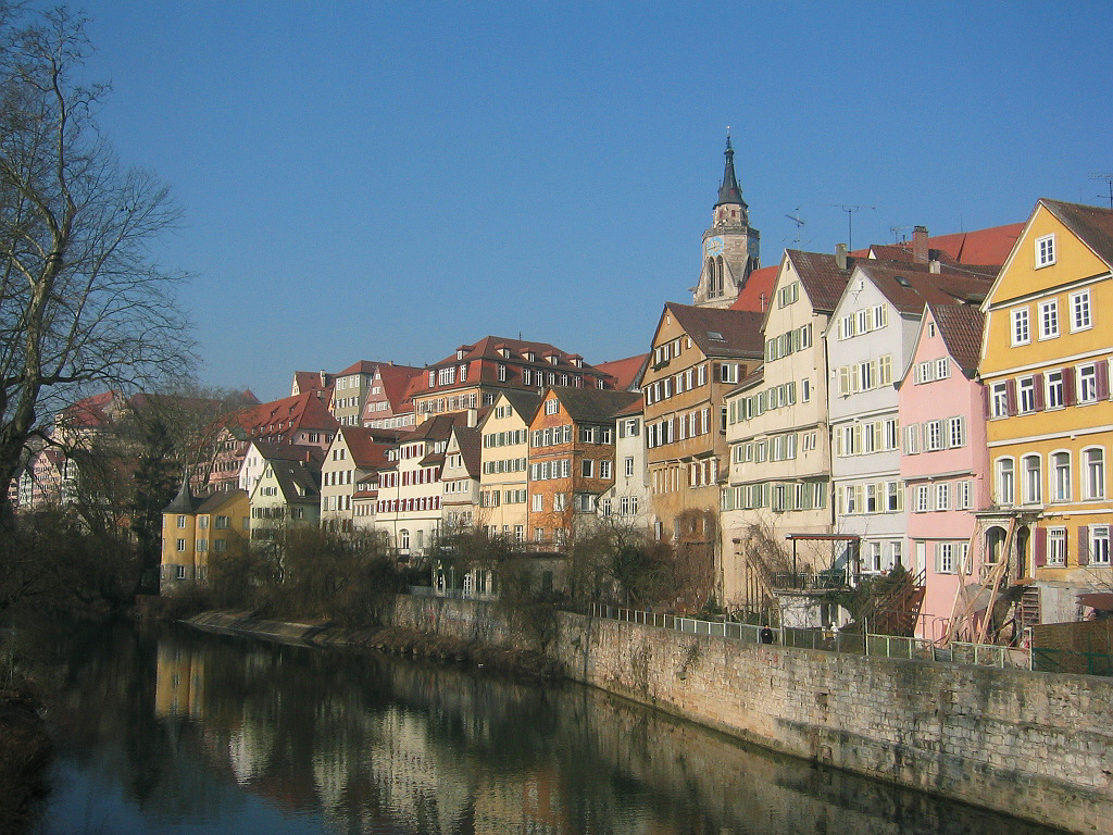 Content image, tubingen
|
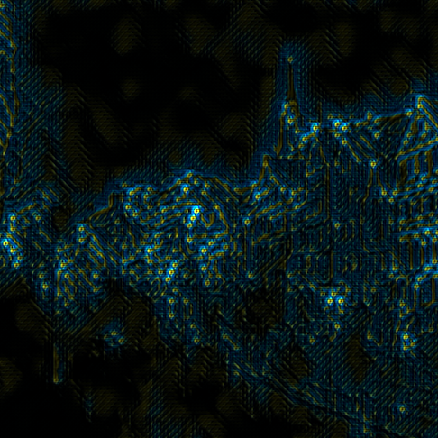 Stylized image, after 1000 iterations of training
|
 Stylized image, after 10000 iterations of training
|
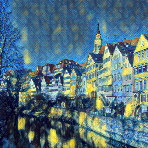 Stylized image, after 30000 iterations of training
|
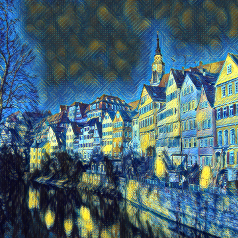
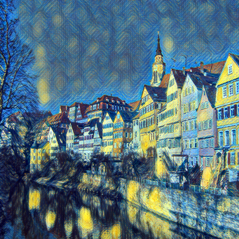 Stylized image, after 40000 iterations of training
|
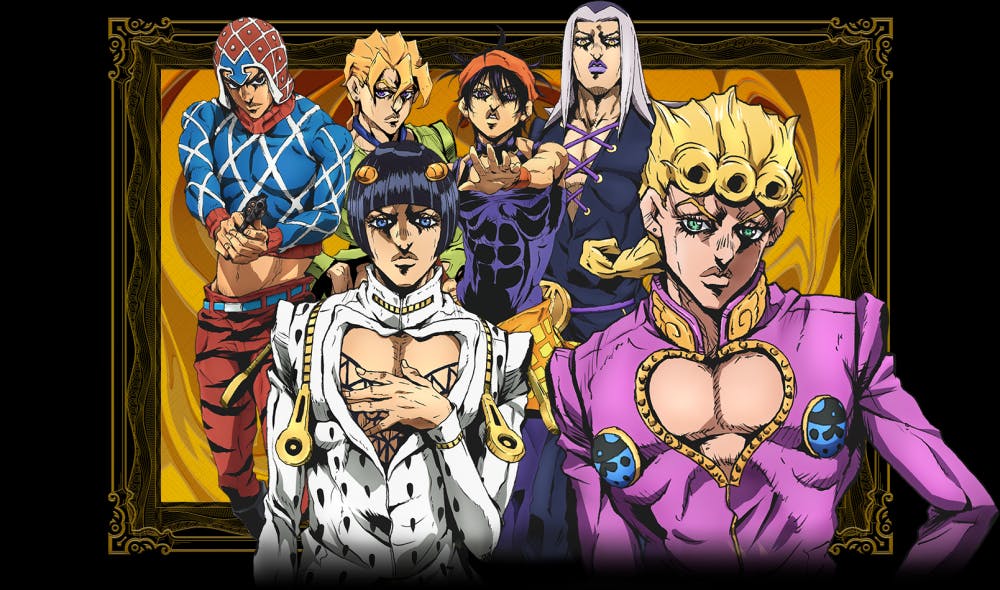 Style image, the Bizarre Adventure of JOJO
|
 Content image, Wally
|
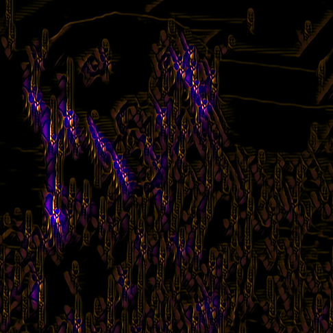 Stylized image, after 1000 iterations of training
|
 Stylized image, after 10000 iterations of training
|
 Stylized image, after 30000 iterations of training
|
 Stylized image, after 40000 iterations of training
|
References
[1] https://cs.stanford.edu/people/jcjohns/papers/eccv16/JohnsonECCV16.pdf
|