 Sketch
 Before optimization
 Optimizing
 Voila!
11-747 Learning-based Image Synthesis Manuel Rodriguez Ladron de Guevara
Sketch
Before optimization
Optimizing
Voila!
This assignment explores different techniques to manipulate images using the GAN latent space. The resulting
edition lies on the manifold of natural images. This assignment has 3 parts: inverting a trained generator
(dcgan or stylegan), interpolation over the latent space, and image editing (scribble to image and editing over
desired image).
Before delving into the assignment details, there are 5 nice references to help understand the nature of the
task:
Generative Visual Manipulation on the Natural Image Manifold
Neural Photo Editing with Introspective Adversarial Networks
Image2StyleGAN: How to Embed Images Into the StyleGAN Latent Space
Analyzing and Improving the Image Quality of StyleGAN
GAN Inversion: A Survey.
This task requires to solve an optimization problem to reconstruct a desired input image from a particular latent
code. Natural images lie on a low-dimensional manifold, and we choose the output manifold of a trained generator
as close to the natural image manifold. We set up the following nonconvex optimization problem:
For some choice of loss $\mathcal{L}$, a trained generator $G$ and a given real image $x$, we can write:
$$z* = argmin_z \mathcal{L}(G(z), x)$$
We choose a combination of pixel loss and perceptual loss, as standard pixel losses alone tend to not work well for
image synthesis tasks. As this is a nonconvex optimization problem where we can access gradients, we can attempt
to solve it with any first-order or quasi-Newton optimization method. An issue here is that these optimizations
can be both unstable and slow, but we can run for several random seeds and get the best.
To recap, content loss is a metric function that measures the content distance between two images at a certain individual layer. Denote the Lth-layer feature of input image X as $X^l$ and that of target content image C as $C^l$. The content loss is defined as the squared L2-distance of these two features: $$L_{content}(\overrightarrow{x}, \overrightarrow{c}, l) = \frac{1}{2}\sum_{i,j}(X_{ij}^l - C_{ij}^l)^2$$ We can select at what level within the VGG-19 network we extract features to represent content. It is known that higher layers capture content better than lower layers, where the content reconstruction at these levels is almost perfect. For the experiments below we found that selecting the first 5 conv layers of the VGG-19 works better.
Pixel loss is straight-forward, we can use L1 or L2 losses over the pixel space. For our experiments, we use L2.
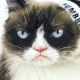
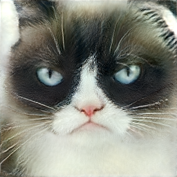
We first compare the result of reconstructing a given cat image with different perceptual layers from a pretrained VGG-19 network. We compare 2 cat images using three different combination of layers. These images are generated using a StyleGAN generator, w+ space a combination of pixel loss and perceptual loss with weights 0.5. All the ablations are done with 1000 iterations using Adam optimizer with a learning rate of 0.003, and L2 regularizer of 0.1.
 Original image
 conv_1_1 to 1_2
 conv_2_1 to 3_2
 conv_1_1 to 3_1
 Original image
 conv_1_1 to 1_2
 conv_2_1 to 3_2
 conv_1_1 to 3_1
We see how lower layers of VGG-19 do not reconstruct the original image properly, producing blurry results, similar to how VAEs output images. Layers beyond the 7th conv layer blow up the reconstruction, so we do not show it here. The difference between using conv 2_1 to 3_2 and using conv 1_1 to 3_1 is minimum. However, using layer 3_2 results in weights explosion for some loss weights, which cause problems for the following ablation studies. We, therefore, use conv 1_1 to 3_1.
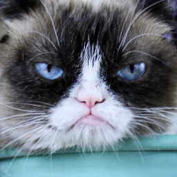
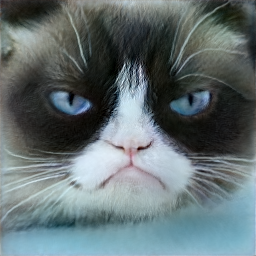
Next, we compare the effect of different weights in each loss:
Original image
 perc w 0, pix w 1
 perc w 0.3, pix w 0.7
 perc w 0.5, pix w 0.5
 perc w 0.7, pix w 0.3
 perc w 1, pix w 0
When setting the weight of perceptual loss to 0, the optimization fails to reconstruct the image. What we see in the second image is something in between the original image generated with the random vector, and the given image (first in the row). Again, the difference between the other settings are not that significant, and judging by the whiskers, we will continue the studies setting the perceptual loss weight to 0.7 and the pixel loss weight to 0.3.
Below, we show the different results using different latent spaces. By column order, w+, w and z. Both w+ and w use StyleGAN model and z uses DCGAN model. Upper row corresponds to averaging 10 vectors and bottom row corresponds to using just 1 vector.
 w+ mean
 w mean
 z mean
 w+ without mean
 w without mean
 z without mean
DCGAN suffers from weight explosion when using the average, while that when using just one vector is able to blurrily reconstruct the image. The best image is yielded by w+ space and averaging across 10 vectors. We can see how the bottom left corner captures the dark spot of the original image, while that using just one vector fails to capture this detail. The optimization time using first-order optimizer of StyleGAN is ~34s, whereas DCGAN optimization time is ~11s. However, using quasi-Newton optimizer of StyleGAN is ~211s.
Original image
Interpolation
 Original image
We use StyleGAN and w+ space to make the interpolations. As we see below, the interpolations between the original images are quite neat, achieving a smooth transition between the 2 given inputs.
 Original image
 Interpolation
 Original image
 Original image
 Interpolation
 Original image
Original image
Original image
 w+ first-order optimizer
w+ quasi-Newton optimizer
w+ first-order optimizer
w+ quasi-Newton optimizer
 Original image
 w+ first-order optimizer
 w+ quasi-Newton optimizer
 Original image
 w+ first-order optimizer
 w+ quasi-Newton optimizer
In this section, we will see the effect of capturing the style of an image using style-space loss. How do we measure the distance of the styles of two images? The Gram matrix is used as a style measurement. Gram matrix is the correlation of two vectors on every dimension. Specifically, denote the k-th dimension of the Lth-layer feature of an image as $f^L_k$ in the shape of (N,K,H∗W). Then the gram matrix is $G=f^L_k(f^L_k)^T$ in the shape of (N, K, K). The idea is that two of the gram matrix of our optimized and predicted feature should be as close as possible.
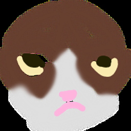
We can treat the scribble similar to the input reconstruction. In this part, we have a scribble and a mask, so we can modify the latent vector to yield an image that looks like the scribble.To generate an image subject to constraints, we solve a penalized non-convex optimization problem. We’ll assume the constraints are of the form $f_i(x)=v_i$ for some scalar-valued functions $f_i$ and scalar values $v_i$. Written in a form that includes our trained generator G, this soft-constrained optimization problem is: $$z* = argmin_z \sum_i || f_i(G(z)) - v_i||^2$$ Given a user color scribble, we would like GAN to fill in the details. Say we have a hand-drawn scribble image $s\inℝ^d$ with a corresponding mask $m\in0,1^d$. Then for each pixel in the mask, we can add a constraint that the corresponding pixel in the generated image must be equal to the sketch, which might look like $m_ix_i$ = $m_is_i$. Since our color scribble constraints are all elementwise, we can reduce the above equation under our constraints to: $$z* = argmin_z \sum_i || M * G(z) - M*S||^2$$ where ∗ is the Hadamard product, M is the mask, and S is the sketch.
We found that adding between 0.01 and 0.1 L2 regularization gave better results using Adam optimizer.
Sketch
Initial latent vector image
Final latent vector image
 Sketch
 Initial latent vector image
 Final latent vector image
 Sketch
 Intitial latent vector image
 Final latent vector image
Sketch
Final latent vector image
Sketch
 Intitial latent vector image
 Final latent vector image
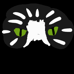
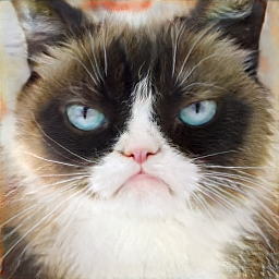
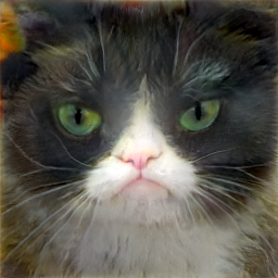
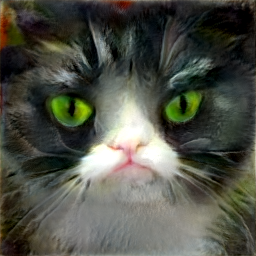
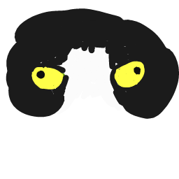
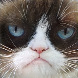
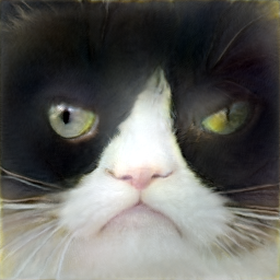
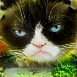
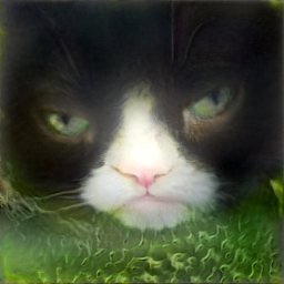
We can first project a latent onto a desired image that we want to edit, and then use the latent corresponding to this image as starting point to edit following a scribble.
Desired image to edit
 Adding green eyes
 Intitial latent vector image
 Final latent vector image
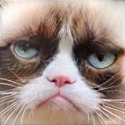
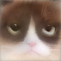
We experiment using high resolution cats. Results below!
 Original image
 Reconstruction
 Original image
 Reconstruction